Polynomial-time algorithms for prime factorization and discrete logarithms on a quantum computer Shor, 1996
We’re sticking with the “Great moments in computing” series again today, and it’s the turn of Shor’s algorithm, the breakthrough work that showed it was possible to efficiently factor primes on a quantum computer (with all of the consequences for cryptography that implies). Wikipedia has a neat timeline of developments in quantum computing which tells us that Shor’s algorithm was actually executed on a real quantum computer for the first time in 2001 – when it factored 15!
The presentation of the algorithm in the paper is hard to follow when you first read it cold, but thankfully there are lots of materials out there which help to bring it to life. Here’s Scott Aaronson’s explanation using only basic math: “Shor, I’ll do it.” I also really enjoyed Kelsey Houston-Edward’s videos in the PBS Infinite Series (danger: you can lose many hours in that YouTube channel!), ‘The Math Behind Quantum Computers’ and ‘Hacking at Quantum Speed with Shor’s Algorithm.’
Beyond the algorithm itself, the paper also touches on interesting discussions around what it is that makes a problem amenable to an efficient solution on a quantum computer, and hence what classes of problems quantum computers may efficiently solve.
In the history of computer science… most important problems have turned out to be either polynomial-time or NP-complete. Thus quantum computers will likely not become widely useful unless they can solve NP-complete problems. Solving NP-complete problems efficiently is a Holy Grail of theoretical computer science which very few people expect to be possible on a classical computer. Finding polynomial-time algorithms for solving these problems on a quantum computer would be a momentous discovery.
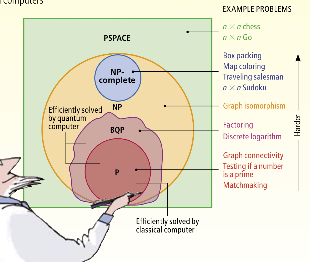
Writing in 1996, Shor saw some ‘weak indications’ that quantum computers would not be able to solve NP-complete problems, but wasn’t yet prepared to rule that possibility out. Scott Aaronson has a wonderful 2008 piece in Scientific American exploring this question, ‘The limits of quantum.’ The key diagram is this one:
For the latest thinking on quantum supremacy and complexity spaces see ‘Complexity-theoretic foundations of quantum supremacy.’
At the outer level we have PSPACE problems – these are problems that a conventional computer can solve using only a polynomial amount of memory, but possibly an exponential number of steps. In other words, they are polynomial in space (PSPACE), but not necessarily in time.
An important subset of PSPACE problems are the NP problems. These are problems whereby it takes a potentially exponential number of steps to find a solution, but once a solution has been found, you can verify that it is indeed a solution in polynomial time.
Within NP there are two further disjoint subsets: NP-complete problems, and P problems. NP-complete problems are a subset of NP problems that all share a fundamental structure. If you can find an efficient algorithm to solve any one of the NP-complete problems, then it is possible to adapt it to also solve any of the others. We have no known algorithm to efficiently (in polynomial time) solve any NP-complete problem. P problems are the subset of NP problems that we do know how to solve efficiently in polynomial time.
That’s the classical computing territory. How do quantum computers impact this landscape? The BQP class of problems (Bounded-error, Quantum, Polynomial time) are those that quantum computers can solve in polynomial time. All P problems are also in BQP (anything a classical computer can solve in polynomial time, so can a quantum computer), and all BQP problems are also in PSPACE (i.e., quantum computers don’t have any silver bullets to offer when it comes to resource consumption). All NP-complete problems are believed to be outside BQP (so quantum computers aren’t going to radically change everything — though Grover’s algorithm does show that we can get a quadratic speed up here). That leaves some problems in BQP that are also in NP, but not in P, where a quantum computer has a real edge over classical computers. These problems can be solved in polynomial time on a quantum computer, but require exponential time on a classical computer. The canonical examples of those problems are factoring integers and discrete logarithms. The quantum algorithms for these problems are the subject of today’s paper choice.
What is it about a problem that places it in BQP \ P?
Through the magic of superposition, a quantum computer with n qubits can be in an arbitrary superposition of up to 
Extending our probability distribution analogy for a moment, so far we’ve been assuming that the distribution is uniform. But the distribution doesn’t have to be uniform. If we can exploit certain global properties of the overall solution space (not just features of point solutions within the space) we may be able to shape the distribution in our favour. In particular, if we can make it more likely that a randomly drawn sample actually is a solution, we can increase our odds of resolving to a solution when we take a measurement. On a physical level, what we want is that non-solutions destructively interfere with each other, and solutions constructively interfere, thus increasing the amplitude of the wave at solution points.
Now all we have to do is run the quantum computation a sufficient number of times, (say 100), and the solutions should rise to the fore because we’ll sample them more often. Problems in BQP \ P are those where we can find something in the overall structure of the solution space that allows us to do this distribution shaping trick.
Shor’s algorithm for factoring primes
Shor’s algorithm uses a little number theory to convert the problem of finding prime factors into an equivalent problem which reveals an overall structure in the solution space we can exploit along the lines we’ve just been discussing.
Our quantum factoring algorithm takes asymptotically
steps on a quantum computer, along with a polynomial (in log n) amount of post-processing time on a classical computer that is used to convert the output of the quantum computer to factors of n.
A 2048-bit key has around 1400 decimal digits. So factoring it should take on the order of (1400^2)*3.14*0.5, or approximately 3 million steps.
Here I’m going to follow Kelsey Houston-Edward’s high-level explanation of the algorithm, which has 4 main steps. Suppose we want to find the prime factors p and q of N. We proceed as follows:
- Pick a random number a less than N. Repeat until you’ve found some a which is not a factor of N.
- Find r, the period of a mod N. (We’ll come back to this in just a moment)
- Check that r is even, and that
.
- Let
, and let
.
Step 2 is both the tricky part (i.e., where we need to take advantage of quantum computation), and also the part that enables us to find and exploit a global property of the solution space. We construct a sequence 

The resulting pattern of digits (2,4,8,1) repeats with a period of 4. So 


Steps 1, 3, and 4 we can do quite efficiently on a classical computer, but step 2 we can’t.
Following Aaronson now:
…suppose we could create an enormous quantum superposition over all the numbers in our sequence: a mod N, a^2 mod N, a^3 mod N, etc. Then maybe there’s some quantum operation we could perform on that superposition that would reveal the period.
The quantum operation that does this for us is the Quantum Fourier Transform (QFT)! This is described in §4 of the paper. Back to Kelsey Houston-Edwards, who has a nice easy to follow explanation in her video starting at 8:50.
Consider a set of dials, with increasing number of points equally spaced on a unit circle:
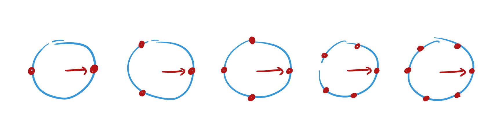
Every dial starts off pointing to 3 o’clock. Now for each number x in the sequence move the hand of each dial one place counter-clockwise. When x = 1, record the positions of the hands. Here are the positions after we’ve processed ‘2,4,8,1’ :
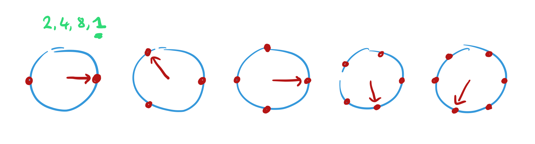
Above each dial we’ve placed a point. Move that point by 1 unit in the direction the hand is pointing to when recording the hand positions..
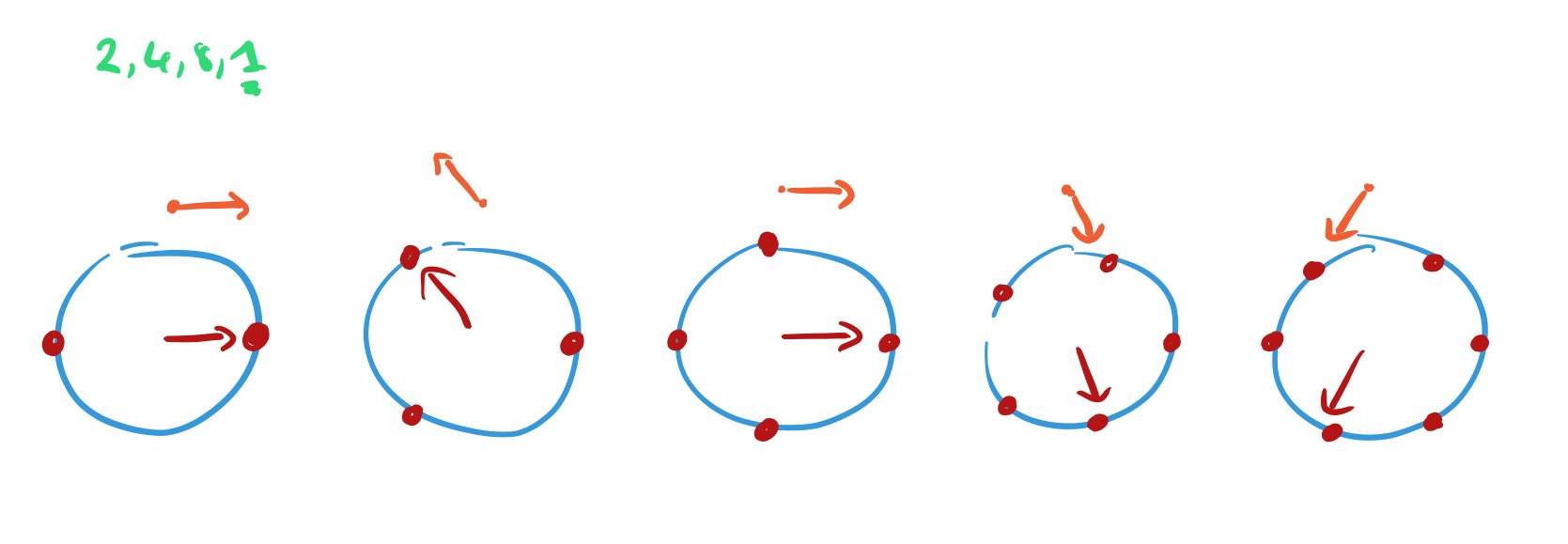
Keep doing this as you move through the sequence, and you’ll find that most of the points just trace out a shape eventually returning to where they started. But the dial with the same number of positions as the period of the sequence will always be pointing in the same direction each time, and it’s path will extend off into the distance.
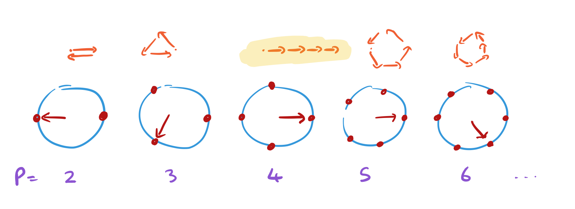
The lengths of the paths traced out are like the amplitudes, or probabilities of the corresponding state. So by following this process, we’ve greatly increased the chances of sampling the right answer.
Following this general principle, the QFT is a linear transform mapping a quantum state encoding a sequence, to a quantum state encoding the period of the sequence.
Back to Aaronson:
Another way to think about this is in terms of interference. I mean, the key point about quantum mechanics — the thing that makes it different from classical probability theory — is that, whereas probabilities are always nonnegative, amplitudes in quantum mechanics can be positive, negative, or even complex. And because of this, the amplitudes corresponding to different ways of getting a particular answer can “interfere destructively” and cancel each other out.
For all periods other than the true one, the amplitude contributions cancel each other out, only for the true period do they all point in the same direction, “and that’s why, when we measure at the end, we’ll find the true period with high probability.”
Section 6 in the paper describes the algorithm for computing discrete logarithms, which also makes use of the QFT, but we’ll leave that for another day!

Just for the record, NP problems can be, and routinely are, solved by conventional computers. SAT solvers routinely solve problems of 10million variables. Asymptotic complexity is a single data point – like a map that describes a mountain range by the height of the highest peak.
For modelling travelling-salesman, use a piece of wood with iron nails, and carve out the roads between the nails, and pour a sufficiently thick magnetic fluid on the roads, until the fluid touches all nails.
Small nitpick, you say
“When searching in a solution space therefore, a quantum algorithm can explore 2^n possible solutions in parallel, in the same total elapsed time as it takes to explore any one solution”
but then in the Scott Aaronson blog he points out
“Hundreds of popular magazine articles notwithstanding, trying everything in parallel just isn’t the sort of thing that a quantum computer can do”
Your path for the unit checks right with 2 dots is wrong. It is not a cycle for period length of two. I am also a bit unsure about the argument as divisors of the period would not trace out.
Also your image for 6 should be a cycle with 3 edges.
Sorry swipe keyboard. Now corrected:
Your path for the unit circle with 2 dots is wrong. It is not a cycle of length of two. I am also a bit unsure about the whole argument as divisors of the period would not trace out; here 2 is such an example.
Also your image for 6 should be a cycle with 3 edges.
The problem with the divisors of the period is not a real problem:
Let r be the period we want to get and let p1*p2*….=r be the prime factorisation of r. Let r'<r be a divisor of the period we measure. Then we start again with a^r' mod n as the next a in the process. With that we guarantee that r' is not measured again. So continuing this procedure on and on we either sieve out all factors of the period (and can compute the product to get r in the end) or we measure the period.