The case for learned index structures Kraska et al., arXiv Dec. 2017
Welcome to another year of papers on The Morning Paper. With the rate of progress in our field at the moment, I can’t wait to see what 2018 has in store for us!
Two years ago, I started 2016 with a series of papers from the ‘Techniques everyone should know’ chapter of the newly revised ‘Readings in Database Systems.’ So much can happen in two years! I hope it doesn’t take another ten years for us to reach the sixth edition of the ‘Red Book,’ but if it does, in today’s paper choice Kraska et al., are making a strong case for the inclusion of applied machine learning in a future list of essential techniques for database systems. I can’t think of a better way to start the year than wondering about this blend of old and new — of established database systems research and machine learning models — and what it all might mean for systems software of the future. I’m going to break my summary up into two posts (today and tomorrow) so that we can focus on the big picture today and dive into the details tomorrow.
The thing I like best about this paper is that it opens the door to a different way of thinking about components of systems software. By cleverly framing the problem of indexing, the authors show the potential to use machine learning deep inside a data management system. There are some constraints in applicability of the current implementation (which we’ll get to), but even then results which show up to 70% speed improvements while simultaneously saving an order-of-magnitude in memory are worth paying attention to. Remember, these improvements are obtained against algorithms which have been tuned over decades. Rather than getting too hung on up the particulars of the indexing use case straight away though, I want to dwell on the bigger picture for a few moments:
…we believe that the idea of replacing core components of a data management system through learned models has far reaching implications for future systems designs and that this work just provides a glimpse of what might be possible.
When does it make sense (in systems software) to replace a hand-engineered data structure and/or algorithm with a machine-learned model? The best analogy I can come up with at present to address this question is personalisation. Early web sites and apps showed the same content to everyone. But today, most sites offer you a highly personalised experience, having found that this works better both for them and (hopefully!) for you. The generic experience might be good, but the personalised experience is better. In this analogy, the equivalent of a user in the world of systems software, is I think, a workload — where a workload is a combination of data & access patterns. And one day we might say something like this: “Early systems software used the same generic configuration, data structures, and algorithms for all workloads. But today, most systems learn from and optimise for the specific workloads they are running.”
An easy to understand example that we looked at a few times last year is configuration: most systems ship with a default configuration that’s ok across a broad set of workloads, but tuning the configuration to suit your specific workload can yield big performance improvements. That’s the pattern I think we’re looking for: workload personalisation makes sense to explore when the performance of the system is sensitive to the characteristics of the particular workload it’s running, and if we had known those characteristics a priori we could have optimised the system for them. Frankly, pretty much all systems software is sensitive to the characteristics of the workload running on it! This puts me very much in mind of the ‘no free lunch theorem’ too: “…if an algorithm performs well on a certain class of problems then it necessarily pays for that with degraded performance on the set of all remaining problems.”
A couple of other considerations come to mind: the workload personalisation needs to occur within some bounded component of the system (one that can be abstracted as a function), and we need a way of preserving guarantees / honouring constraints. Consider the use of probabilistic data structures today, where we’re already comfortable with the fact that they’re approximations (as a learned function will be). Perhaps the best known is the Bloom filter, which tells us whether or not an element is likely to be in a set. Bloom filters come with an important guarantee – there are no false negatives. Learning a function that has ‘only a small probability’ of a false negative is not the same at all in many use cases. It turns out the authors have a really neat solution to this problem that we’ll look at tomorrow!
Unlocking the full potential of workload personalisation needs an online learning/optimisation approach, since:
the engineering effort to build specialized solutions for every use case is usually too high… machine learning opens up the opportunity to learn a model that reflects the patterns and correlations in the data.
In this paper, the approach is applied to the automatic synthesis of specialized indexed structures, which the authors term learned indexes.
On CPUs, GPUs, and TPUs
The implementations in this paper were done using CPUs, but there’s another reason why neural net style models will become increasingly attractive in the future: they can run very efficiently on GPUs and TPUs. While CPUs are plateauing in performance, NVIDIA predict a 1000x increase in GPU speed by 2025. With closer integration of CPU/GPU/TPU units to reduce the handover costs, the GPU/TPU performance curve looks to be the one to ride to achieve maximum performance into the next decade.
Introducing learned (range) indexes
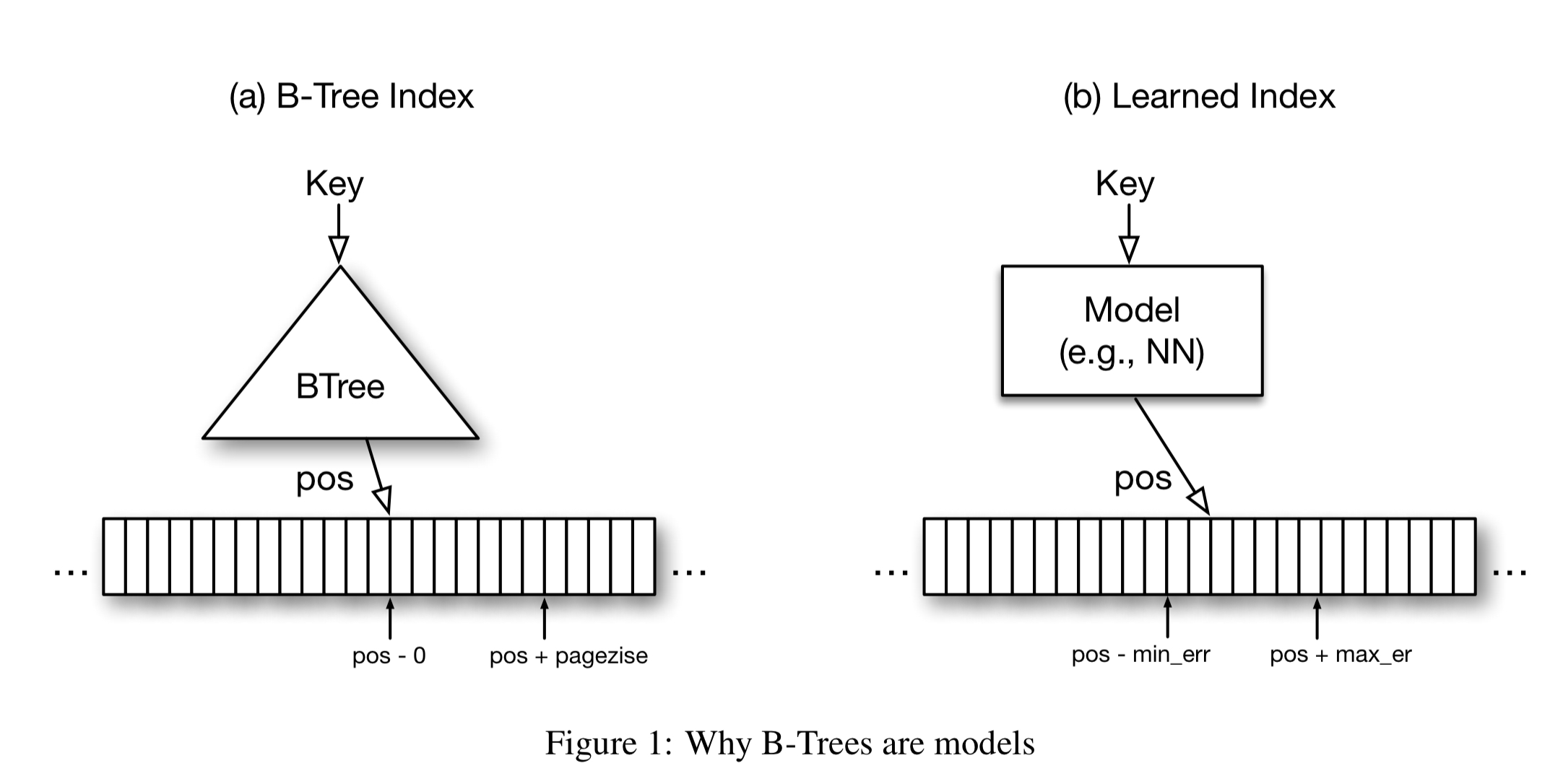
This paper is primarily concerned with read-only in-memory analytical workloads. In a typical B-Tree index found in an analytics database today, the B-Tree provides a mapping from a lookup key to a position inside a sorted array of records. The index contains entries for every nth key, for example, the first key in a page. The guarantee from such a B-Tree is that the key will be found within ‘page-size’ of the returned location, if it exists. It’s a function from key to location, with error bound guarantees. We can learn a function, but what about the guarantees?
At first sight it may be hard to provide the same error guarantees with other types of ML models, but it is actually surprisingly simple. The B-tree only provides this guarantee over the stored data, not for all possible data. For new data, B-Trees need to be re-balanced, or in machine learning terminology re-trained, to still be able to provide the same error guarantees. This significantly simplifies the problem: the min- and max-error is the maximum error of the model over the training (i.e. the stored) data.
If we execute the model for every key, and remember the worst over- and under-predictions, then we know that a lookup for any key that exists must fall within these bounds. Using a machine learned model becomes possible therefore, and transforms an O(log n) B-Tree look-up into a constant operation.

Traversing a single B-Tree page of size 100 takes roughly 50 cycles (with any cache-misses), and we would need log100N of those traversals for a lookup in a table with N keys. In comparison, you can do 1 million neural net operations in 30 cycles on NVIDIAs latest Tesla V100 GPU. On modern CPUs we have a budget of about log100N 400 arithmetic operations to beat the B-Tree.
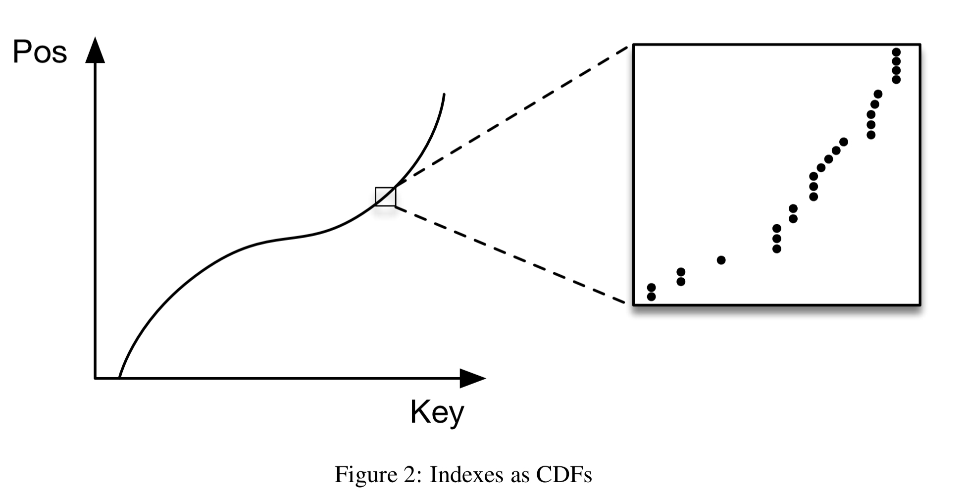
A model that predicts the position of a key within a sorted array is effectively approximating the cumulative distribution function (CDF):

…estimating the distribution for a data set is a well-known problem and learned indexes can benefit from decades of research.
A naive first implementation using a two-layer fully-connected neural network with 32 neurons per layer achieved approximately 1250 predictions per second. The B-Tree was still 2-3x faster though! Why?
- The Tensorflow invocation overhead (especially with a Python front-end) is too great.
- B-Trees ‘overfit’ the data very effectively. In contrast, a learned CDF works well to approximate the general shape, but doesn’t do so well at the individual data instance level (as shown in the callout in the figure above). “Many datasets have exactly this behaviour: from the top the data distribution appears very smooth, whereas as we zoom in more, the harder it is to approximate the CDF because of the randomness on the individual level.” This makes the ‘last mile’ tougher for single neural nets.
- Instead of minimising the average error (typical for ML optimisation), we really want to minimise the min- and max-error bounds.
- B-Trees are extremely cache efficient, whereas standard neural nets are less so.
If we stopped here of course, it wouldn’t be much of a story. But in tomorrow’s post we’ll look at the learning index framework (LIF) which the authors develop to overcome these problems. In addition to range indexes, we’ll also take a look at point indexes (essentially, learned alternatives to hash maps), and existence indexes (learned alternatives to Bloom filters).
Thanks in advance for the upcoming year! Today’s post is definitely a strong start.
Great post. Effectively using ML to personalize systems towards workloads is a great area to explore.