Statistically rigorous Java performance evaluation

Statistically rigorous Java performance evaluation Georges et al., OOPSLA’07

This paper won the 10-year most influential paper award at OOPSLA this year. Many of the papers we look at on this blog include some kind of performance evaluation. As Georges et al., show, without good experimental design and statistical rigour it can be hard to draw any firm conclusions, and worse you may reach misleading or incorrect conclusions! The paper is set in the context of Java performance evaluation, but the lessons apply much more broadly.

Benchmarking is at the heart of experimental computer science research and development… As such, it is absolutely crucial to have a rigorous benchmarking methodology. A non-rigorous methodology may skew the overall picture, and may even lead to incorrect conclusions. And this may drive research and development in a non-productive direction, or may lead to a non-optimal product brought to market.

A good benchmark needs a well chosen and well motivated experimental design. In addition, it needs a sound performance evaluation methodology.

… a performance evaluation methodology needs to adequately deal with the non-determinism in the experimental setup… Prevalent data analysis approaches for dealing with non-determinism are not statistically rigorous enough.

In the context of Java sources of non-determinism can include JIT compilation, thread scheduling, and garbage collection for example. For many benchmarks run today on cloud platforms, non-determinism in the underlying cloud platform can also be a significant factor.

Problems with performance evaluations

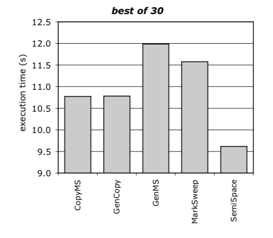
Common at the time of publication (it would be interesting to do a similar assessment of more recent papers) was a method whereby a number of performance runs – e.g. 30 – would be done, and the best performance number (smallest execution time) reported. This was in accordance with SPECjvm98 reporting rules for example. Here’s an example of doing this for five different garbage collectors.

CopyMS and GenCopy seem to perform about the same, and SemiSpace clearly outperforms GenCopy.

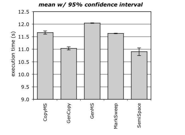
Here are the same experiment results, but reported using a statistically rigorous method reporting 95% confidence intervals.

Now we see that GenCopy significantly outperforms CopyMS, and that SemiSpace and GenCopy have overlapping confidence intervals – the difference between them could be simply due to random performance variations in the system under measurement.

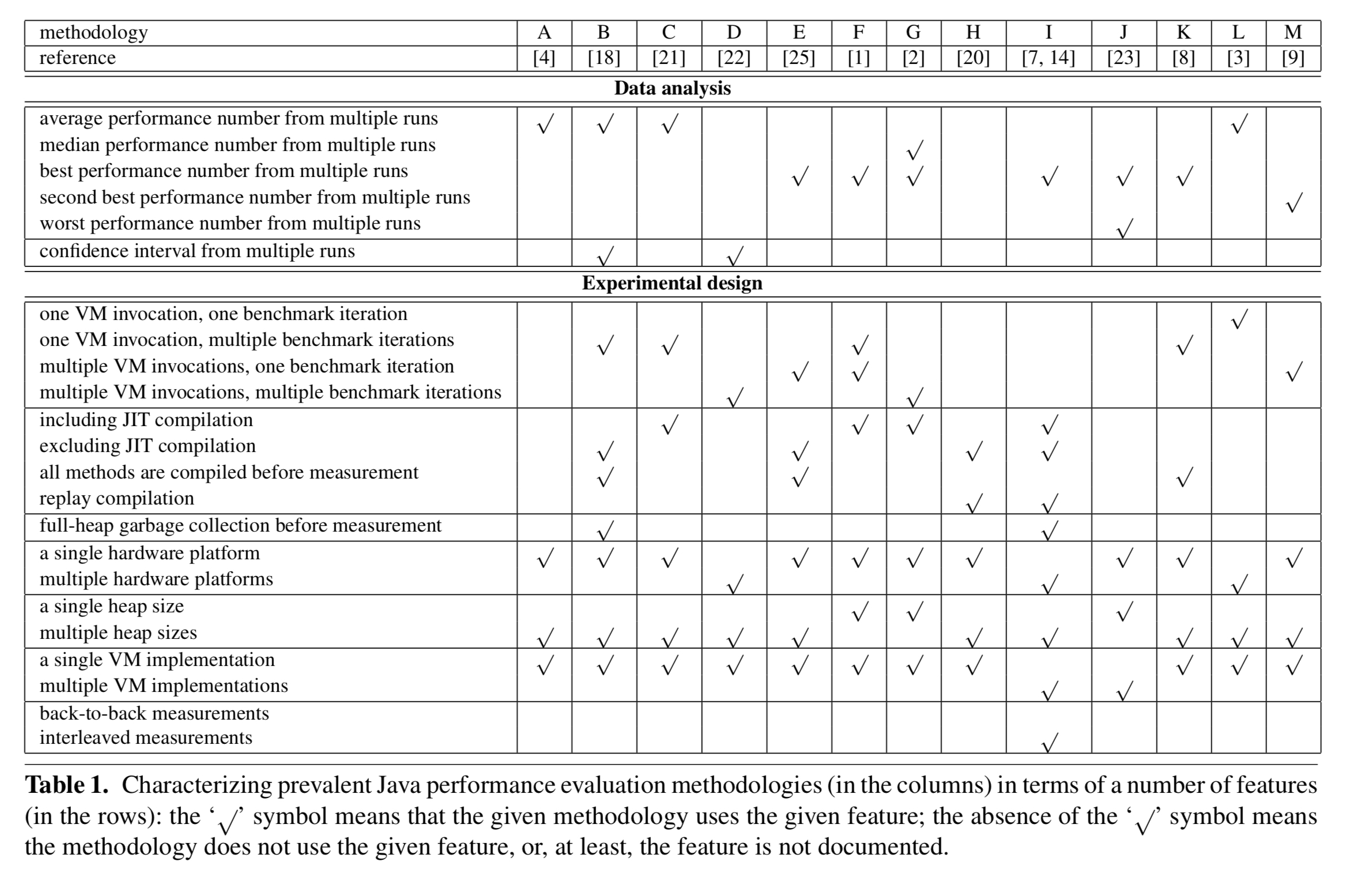
After surveying 50 Java performance papers the authors conclude that there is little consensus on what methodology to use. Table 1 below summarises some of the methodologies used in those papers:

Examples of misleading results

Suppose you use a non-rigorous methodology and report a single number such as best, average, worst etc., out of a set of runs. In a pairwise comparison, you might say there was a meaningful performance difference if the delta between the two systems was greater than some threshold $\theta$ . Alternatively, using a statistically rigorous methodology and reporting confidence intervals, it may be that you see:

overlapping intervals
non-overlapping intervals, in the same order as the non-rigorous methodology
non-overlapping intervals, in a different order to the non-rigorous methodology

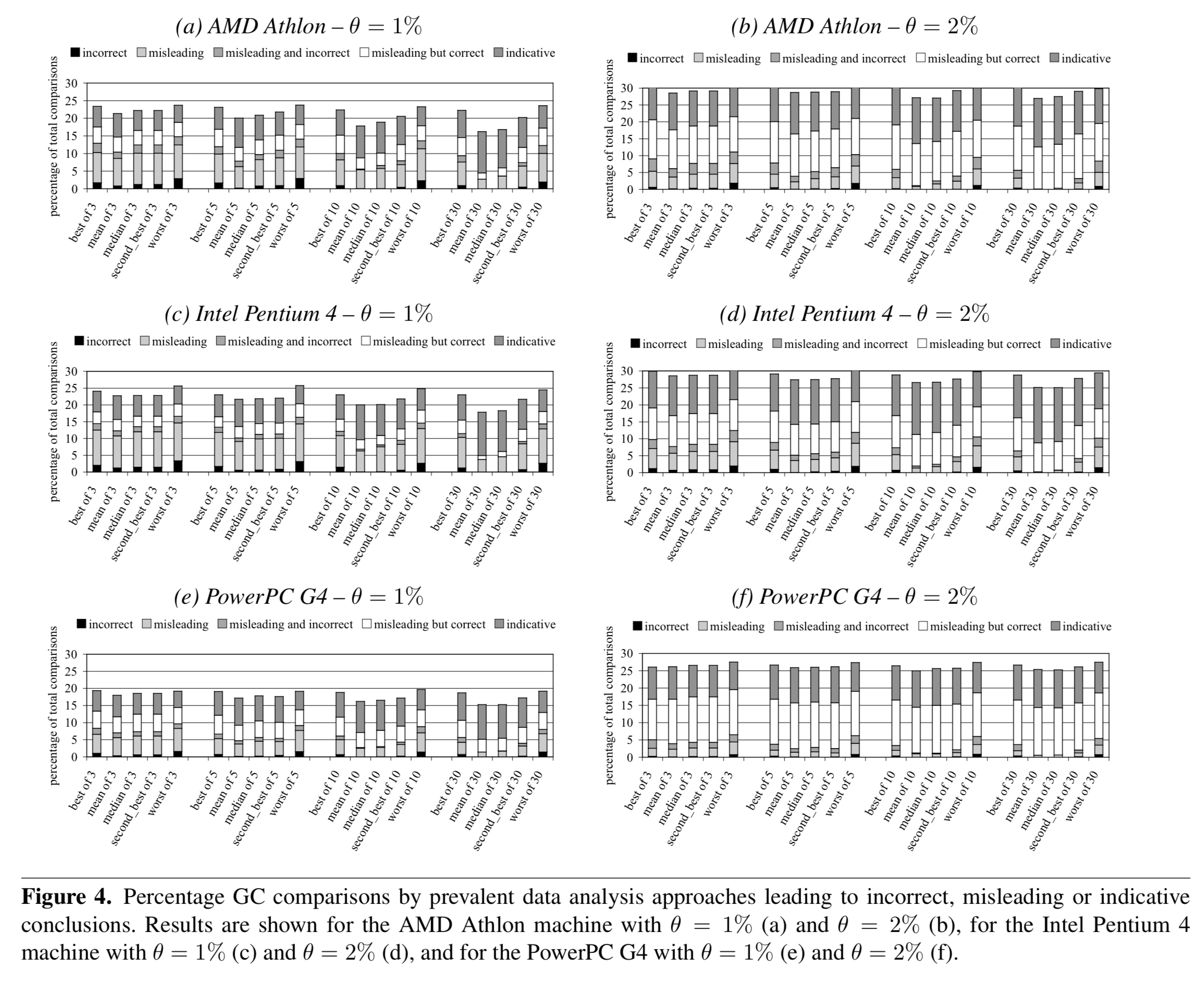
This leads to six different cases – in only one of which can you truly rely on the results from the non-rigorous approach:

The authors run a series of tests and find that all prevalent methods can be misleading in a substantial fraction of comparisons between alternatives – up to 16%. Incorrect conclusions even occur in up to 3% of comparisons. (And if you really must report a single number, mean and median do better than best, second best, or worst).

There are many more examples in section 6 of the paper.

Statistics to the rescue

We advocate adding statistical rigor to performance evaluation studies of managed runtime system, and in particular Java systems. The motivation for statistically rigorous data analysis is that statistics, and in particular confidence intervals, enable one to determine whether differences observed in measurements are due to random fluctuations in the measurements or due to actual differences in the alternatives compared against each other.

Section 3 in the paper is my favourite part, and it essentially consists of a mini-stats tutorial for people doing benchmarks.

If we could get an exact repeatable number out of every performance run, life would be much more straightforward. Unfortunately we can’t do that due to non-determinism (‘random errors’) in the process. So we need to control for perturbing events unrelated to what the experiment is trying to measure. As a first step, the authors recommend discarding extreme outliers. With that done, we want to compute a confidence interval.

In each experiment, a number of samples is taken from an underlying population. A confidence interval for the mean derived from these samples then quantifies the range of values that have a given probability of including the actual population mean.

A confidence interval $[c_1, c_2]$ is defined such that the probability of $\mu$ being between $c_1$ and $c_2$ equals $1 - \alpha$ , where $\alpha$ is the significance level and $(1 - \alpha)$ is the confidence level.

A 90% confidence interval means that there is a 90% probability that the actual distribution mean of the underlying population is within the confidence interval. For the same data, if we want to be more confident that the true mean lies within the interval, say a 95% confidence interval, then it follows that we would need to make the interval wider.

Ideally we would take at least 30 samples such that we can build upon the central limit theorem. With a target significance level $\alpha$ chosen in advance, we can then determine $c_1$ and $c_2$ so that the probability of the true mean being in the interval equals $1 - \alpha$ . It looks like this:

Where $s$ is the standard deviation of the sample, $\bar{x}$ the mean, and $z_{1 - \alpha / 2}$ is obtained from a pre-computed table.

A basic assumption made in the above derivation is that the sample variance $s^2$ provides a good estimate of the actual variance $\sigma^2$ … This is generally the case for experiments with a large number of samples, e.g., $n \geq 30$ . However, for a relatively small number of samples, which is typically assumed to mean $n < 30$ , the sample variance $s^2$ can be significantly different from the actual variance $\sigma^2$ .

In this case, we can use Student’s t-distribution instead and compute the interval as:

The value $t_{1 - \alpha / 2;n-1}$ is typically obtained from a pre-computed table. As the number of measurements $n$ increases the Student t-distribution approach the Gaussian distribution.

Comparing alternatives

Thus far we know how to compute confidence intervals for the mean of a single system. If we compare two system and their confidence intervals overlap, then we cannot conclude that the differences seen in the mean values are not due to random fluctuations in the measurements. If the confidence intervals do not overlap, we conclude that there is no evidence to suggest that there is not a statistically significant difference.

The paper shows the formula for computing a confidence interval for the difference of two means (see section 3.3). If this interval includes zero, we can conclude, at the confidence level chosen, that there is no statistically significant difference between the two alternatives.

If we want to compare more than two alternatives, then we can use a technique called Analysis of Variance (ANOVA).

ANOVA separates the total variation in a set of measurements into a component due to random fluctuations in the measurements and a component due to the actual differences among the alternatives… If the variation between the alternatives is larger than the variation within each alternative, then it can be concluded that there is a statistically significant difference between the alternatives.

The ANOVO test doesn’t tell which of the alternatives the statistically significant difference is between, if there is one! The Tukey HSD (Honestly Significantly Different) test can be used for this.

With ANOVA we can vary one input variable within an experiment. Multi-factor ANOVA enables you to study the effect of multiple input variables and all their interactions. Multivariate ANOVA (MANOVA) enables you to draw conclusions across multiple benchmarks.

Recommendations

Using the more complex analyses, such as multi-factor ANOVA and MANOVA, raises two concerns. First, their output is often non-intuitive and in many cases hard to understand without deep background in statistics. Second, as mentioned before, doing all the measurements required as input to the analyses can be very time-consuming up to the point where it becomes intractable.

Section 4 of the paper therefore introduces a practical yet still statistically rigorous set of recommendations for Java performance evaluation.

To measure start-up performance:

Measure the execution time of multiple VM invocations, each running a single benchmark iteration.
Discard the first VM invocation and retain only the subsequent measurements. This ensures libraries are leaded when doing the measurements.
Compute the confidence interval for a given confidence level. If there are more than 30 measurements, use the standard normal $z$ -statistic, otherwise use the Student $t$ -statistic.

To measure steady-state performance:

Consider $p$ VM invocations, each invocation running at most $q$ benchmark iterations. Suppose we want to retain $k$ measurements per invocation.
For each VM invocation $i$ determine the iteration $s_i$ where steady-state performance is reached, i.e., once the coefficient of variation (std deviation divided by the mean) of the $k$ iterations ( $s_i -k$ to $s_i$ ) falls below a preset threshold, say 0.01 or 0.02.
For each VM invocation, compute the mean $\bar{x}_i$ of the $k$ benchmark iterations under steady-state: $x_i = \sum_{j= s_i-k}^{s_i} x_{ij}$ .
Compute the confidence interval for a given confidence level across the computed means from the different VM invocations. The overall mean $\bar{x} = \sum_{i=1}^{p} \bar{x_i}$ , and the confidence interval is computed over the $\bar{x}_i$ measurements.