ActiveClean: Interactive data cleaning for statistical modeling Krishnan et al., VLDB 2016

Yesterday we saw that one of the key features of a machine learning platform is support for data analysis, transformation and validation of datasets used as inputs to the model. In the TFX paper, the authors reference ActiveClean as an example of data cleaning best practices. And so that’s what we’re going to be looking at today.

Although it is often overlooked, an important step in all model training pipelines is handling dirty or inconsistent data including extracting structure, imputing missing values, and handling incorrect data.

The most common practice for cleaning datasets used in machine learning is to alternate between cleaning and analysis, and goes something like this:

• build and train a model and see how well it does
• find yourself a little disappointed with the accuracy
• examine a few of the records that are wrongly classified, see that they contain errors of some kind (corrupted fields, missing values, etc.), and patch them up
• retrain the model, and repeat…

If you’re doing it this way, you could be seriously undermining your machine learning efforts.

Unfortunately, for statistical models, iteratively cleaning some data and ret-training on a partially clean dataset can lead to misleading results in even the simplest models.

There are two main takeaways for me in this paper, (1) a much better understanding of the ways in which dirty records and attempts to clean them can impact machine learning outcomes, and (2) the ActiveClean approach to solving the problem, which gives you the benefits of iterative improvement while avoiding the pitfalls of naive cleaning.

Cleaning datasets the ActiveClean way versus the traditional iterative way can improve model accuracy by up to 2.5x for the same amount of data cleaned!

The dangers of iterative model cleaning

Let’s start out by getting an intuition for the dangers in iterative cleaning by examining a very simple linear regression problem with just one variable. In the figure below, we have a systematic bias in the variable’s values, causing them to be left-shifted from the true (clean) values:

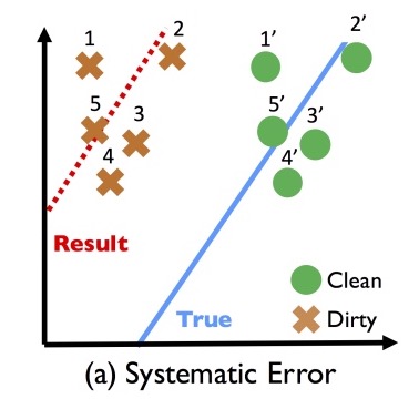
If we try to learn a classifier from this dirty data, then clearly it won’t perform well on clean data.

Suppose we inspect a sample of the data points, discover the bias and fix it. We might end up with a dataset that looks like this:

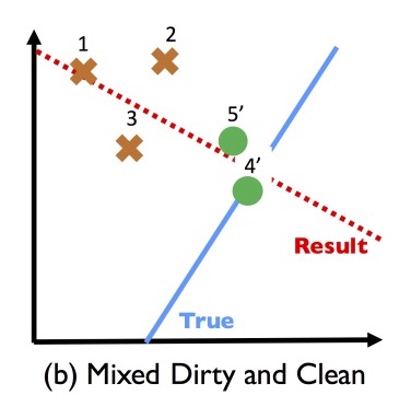
Learning a classifier on this mix ends up being less accurate than if we hadn’t cleaned any records at all!

So what if instead of doing that, we sample a subset of records, clean those, and then train a model on just the cleaned records? That’s not guaranteed to work out well either!

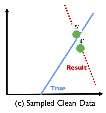
These effects are caused by Simpson’s paradox.

The straightforward application of data cleaning is to repair the corruption in-place, and re-train the model after each repair. However, this process has a crucial flaw, where a model is trained on a mix of clean and dirty data . It is known that aggregates over mixtures of different populations of data can result in spurious relationships due to the well-known phenomenon called Simpson’s paradox. Simpson’s paradox is by no means a corner case, and it has affected the validity of a number of high profile studies.

If naive iterative cleaning has so many risks, you might be tempted to ask why clean at all? Jumping ahead to the evaluation for a moment, here’s an example from training a classifier on the MNIST dataset (images of digits from 0-9). The authors add simulated corruptions to the 5% of the dataset, mimicing standard corruptions in image processing, such as occlusion and low-resolution. Consider the 5×5 removal corruption that deletes a random 5×5 pixel block (sets the pixel values to 0).

Even though these corruptions are generated independently of the data, the 5×5 Removal propagates through the pipeline as a systematic error. The image features are constructed with edge detectors, which are highly sensitive to this type of corruption. Digits that naturally have fewer edges than others are disproportionately affected…

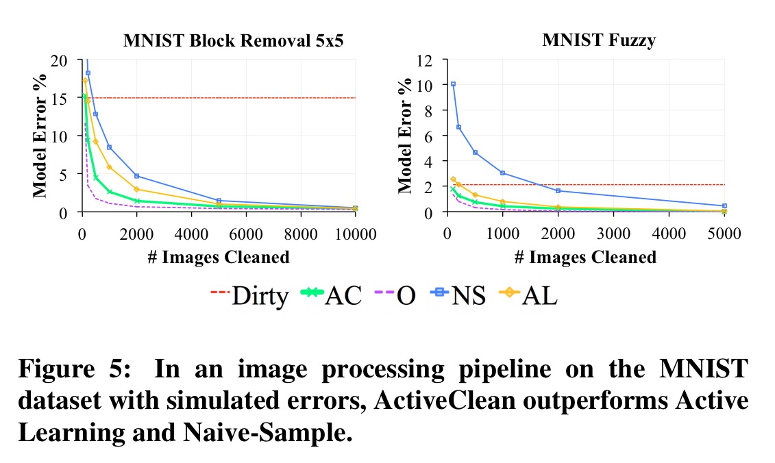
Here you can see that with the random 5×5 removal corruptions (Dirty), the best accuracy the model can achieve is around 85%. In the Optimal (O) conditions – all data is clean – the model converges quickly to much higher accuracy. Active Cleaning (AC), which we’ll look at next gets us much closer to the optimal results, reaching 2% error after examining around 2,200 images out of the 60,000 in the dataset.

Iterative model cleaning done right with ActiveClean

From a statistical perspective, our key insight is to treat the cleaning and training iteration as a form of Stochastic Gradient Descent, an iterative optimization method. We treat the dirty model as an initialization, and incrementally take gradient steps (cleaning a sample of records) towards the global solution (i.e., the clean model). Our algorithm ensures global convergence with a provable rate for an important class of models called convex-loss models which include SVMs, Linear Regression, and Logistic Regression.

ActiveClean assumes records are cleaned on a record-by-record basis, with a user-defined function C, which when applied to a record r can either recover a unique cleaned record r’, or remove the record. C could be implemented in software, or it could be manual action by a human analyst. The ActiveClean architecture includes a Sampler, Cleaner, Updater, Detector, and Estimator.

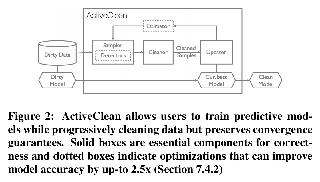
The system is initialised by training on the original (dirty) data, yielding an initial model .

• The Sampler then selects a batch of data that has not been cleaned already. This must be done in a randomised way to ensure convergence, but you can assign higher probabilities to some data, so long as no data has zero sampling probability. A user-provided Detector (optional) can be used to identify records that are more likely to be dirty, thus improving the likelihood that a sample contains true dirty records. From the dirty records detected by the Detector, the very most valuable ones to clean are those which will make the largest impact during optimisation. But how do we know which ones they are? An optional Estimator connects the Detector and the Sampler, providing an estimate of the cleaned data gradient given a dirty record and the dirty gradient.
• The user-provided Cleaner then executes C for each sampled record and outputs their cleaned versions.
• The Updater uses the cleaned batch to update the model using a gradient descent step.
• If a stopping condition has been reached (training error convergence, or maximum number of iterations) then the algorithm terminates, otherwise we proceed to generate the next sample.

Detectors may be rule-based, or alternatively they can be learned by training a classifier as the human analyst selectively modifies data. “The precision and recall of this classifier should be tuned to favour classifying a record as dirty to avoid falsely moving a dirty record into the clean set.” The Estimator works by computing a first-order Taylor Series expansion of the gradient relying on the average change in each feature value (details in section 6.2).

Why ActiveClean works – intuition

Given a newly cleaned batch of data, ActiveClean needs to update the model with a monotone convergence guarantee such that more cleaning implies a more accurate model. Furthermore, ActiveClean needs to select the next batch of data to clean in such a way that the model converges in the fewest iterations possible.

The update algorithm intuitively follows from the convex geometry of the problem. Consider the problem in one dimension…

Here’s an example of the situation when we’ve trained on dirty data:

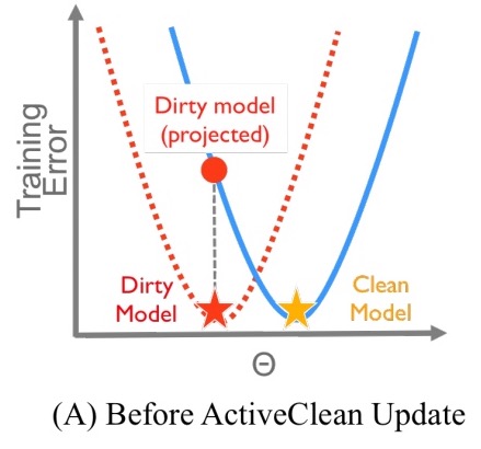
The red dotted line is the loss function on the dirty data, and optimising finds the point at the red star. The true loss function (were the data clean) is represented by the blue line. If we connect the red star vertically to the blue line, we can see that the optimal value on the dirty data, is a suboptimal point on the clean curve. If we had clean data, the true optimal value is represented by the yellow star.

To get closer to the true optimum, the first question is whether to move right or left from the red star.

For this class of models, given a suboptimal point, the direction to the global optimum is the gradient of the loss function. The gradient is a p-dimensional vector function of the current model and the clean data… At the optimal point, the magnitude of the gradient will be zero. So intuitively, this approach iteratively moves the model downhill (transparent red circle) – correcting the dirty model until the desired accuracy is reached.

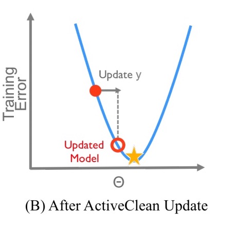
The gradient depends on the clean data of course, which we don’t have! But we can approximate the gradient from a sample of newly cleaned data. This estimate is a combination of the gradient from the already cleaned data, and a gradient estimate from the sample of dirty data to be cleaned, weighting the cleaned records in the sample by their respective sampling probabilities.

Formal proof that this method provides an unbiased estimate of the true gradient is provided in a supplementary technical report.

Experimental results

The evaluation section compares ActiveCleaning against an Oracle (O) with complete access to the ground truth, a Naive-Sampling (NS) approach which draws a random sample to clean and trains over the set of records that have been cleaned so far, and a Naive-Mix (NM) approach which draws a random sample to clean, merges the cleaned data, and trains over the whole dataset. Experiments are done with a couple of relational datasets (IMDB, and the “Dollars for Docs” dataset from ProPublica), MNIST, and two machine learning benchmark datasets: an income classification task, and a seizure classification task.

On the relational data, ActiveClean converges faster that the non-oracle alternatives, and gives better accuracy.

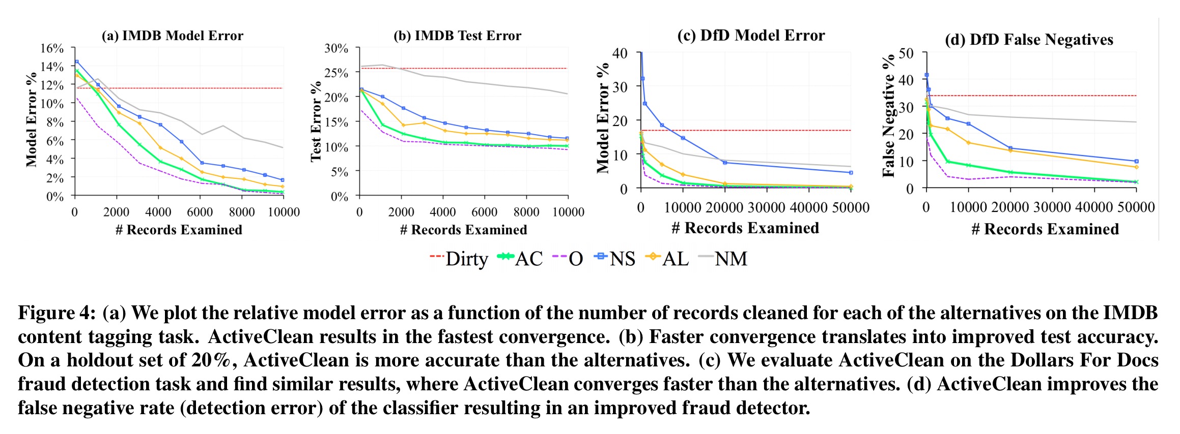
We see similar results with MNIST as discussed earlier, and with the machine learning benchmarks:

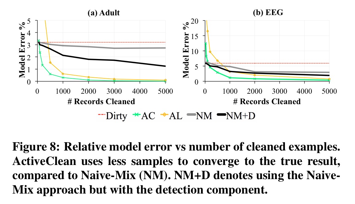
The results show that our proposed optimizations can improve model accuracy by up-to 2.5x for the same amount of data cleaned. Furthermore for a fixed cleaning budget and on all real dirty datasets, ActiveClean returns more accurate models than uniform sampling and Active Learning [Active Learning iteratively selects the most informative unlabeled examples to label in partially labeled datasets].