Luck is hard to beat: the difficulty of sports prediction Aoki et al., KDD’17
You can build all the outcome prediction models you like, such as the strategic play model we looked at yesterday, but some events have a certain amount of inherent unpredictability.
There have been empirical and theoretical studies showing that unpredictability cannot be avoided. Indeed, Martin et al., showed that realistic bounds on predicting outcomes in social systems imposes drastic limits on what the best performing models can deliver. And yet, accurate prediction is a holy grail avidly sought in financial markets, sports, arts and entertainment award events, and politics.
In ‘Luck is hard to beat’ the authors try to quantify the amount of inherent unpredictability in sports: i.e., how much of the outcome is due to luck, and how much due to skill? They look at data from 1,503 seasons across a variety of sports from 2007 to 2016. All the sports selected use a round-robin system where every team plays every other team twice: once at home and once away. In total we’re looking at: 42 leagues, and 310 seasons of basketball; 51 leagues and 328 seasons of volleyball; 25 leagues and 234 seasons of handball; and 80 leagues and 631 seasons of soccer.
The first step is the development of a skill coefficient, φ that indicates how far the results of a season (tournament) are from what would be expected if the competition was based on pure luck. Then for competitions that do seem to have a significant skill component, the paper examines how many teams need to be removed from the competition for it to return to an essentially random situation. It took me until quite deep into the paper to get an intuition for what this was really saying. Take an example from the English Premier League: for the seasons between 2007 to 2016 the average number of teams you need to remove is 4.9. Manchester United appeared in that list 9 out of the 10 seasons, and other teams appeared as often as 7 times in that list. So what this is saying is that if you take out a small number of the top clubs (relegation deals with the bottom clubs), then the remaining places are pretty much a random outcome. The final part of the paper looks at a Bayesian model of skills for NBA, one of the sports in which skill is shown to have a larger degree of influence on the outcome. Using the model, we can estimate the likelihood that the underdog (lesser skilled team) wins in a given game: 45% chance when playing at home, and 27% chance when playing away.
Modelling a skill coefficient
… our aim is to define a metric by which performance can be assessed with respect to a baseline where the teams have the same ability or skill and the tournament is determined by pure chance.
The authors build their model up step by step in a nice intuitive way. Let’s begin:
- Let
be a random variable representing the points earned by a team when it plays in a match at home, and
be the points earned when it plays away. The distributions will be different for different sports. In football (soccer) for example it’s 3 points for a win, 1 for a draw, and 0 for a loss, regardless of whether you’re playing home or away.
- Let
,
, and
be the probabilities that a home team wins, draws (ties) or loses respectively.
- The expected value of
, and variance is
. (And the similarly for the expected value of
Now let’s think about a tournament setting with 


is therefore the total random score a given team obtains at the end of a tournament.
If all teams had equal skill, after k matches at home and k away matches, the distribution of final scores
would follow approximately a normal distribution with parameters
and
. This represents our baseline model, against which the observed empirical results are to be contrasted.
- For each season, we have the observed value of
for each team (i.e., we know how many points they scored!), so we can calculate the empirical variance
.
- And finally, we can compare the observed variability to the expected value under the equal skills assumption:

Which gives us a skills coefficient 
![[-\inf, 1]](https://s0.wp.com/latex.php?latex=%5B-%5Cinf%2C+1%5D&bg=eeeeee&fg=666666&s=0&c=20201002)
The balance between luck and skills in different sports
So after all this, what does the data say? For the sports investigated, basketball is the sport where skill plays the larges part, followed by volleyball, soccer, and then handball.
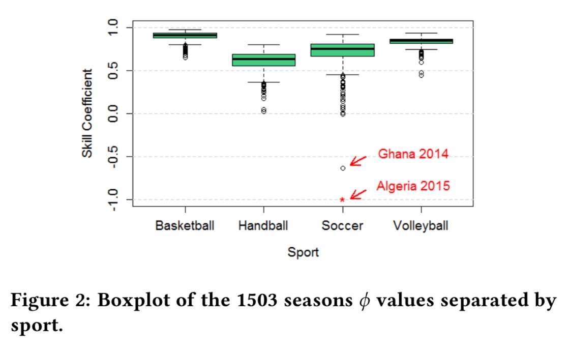
A possible explanation:
… players usually score many points in basketball and volleyball games. Due to the long sequence of relevant events, it is more difficult for a less skilled team to win a game out of pure luck. However, in soccer and handball there are much less relevant events leading to points… This makes it easier for a less skilled team to win a match due to a single lucky event.
All basketball leagues had a strong skill component in their final results, whereas in soccer luck can be a dominant factor in as many as 7.13% of seasons.
Even in basketball though, skill doesn’t completely determine the final ranking.
In each season, some teams have more extreme skills while the others have approximately the same skill level. It is that first group that drives the
coefficient words and close to its maximum value. Where they absent, the season would resemble a lottery.
So how many teams need to be removed from various leagues/seasons in order to make it appear random? I.e., how many sufficiently skills-differentiated teams are there in such leagues?
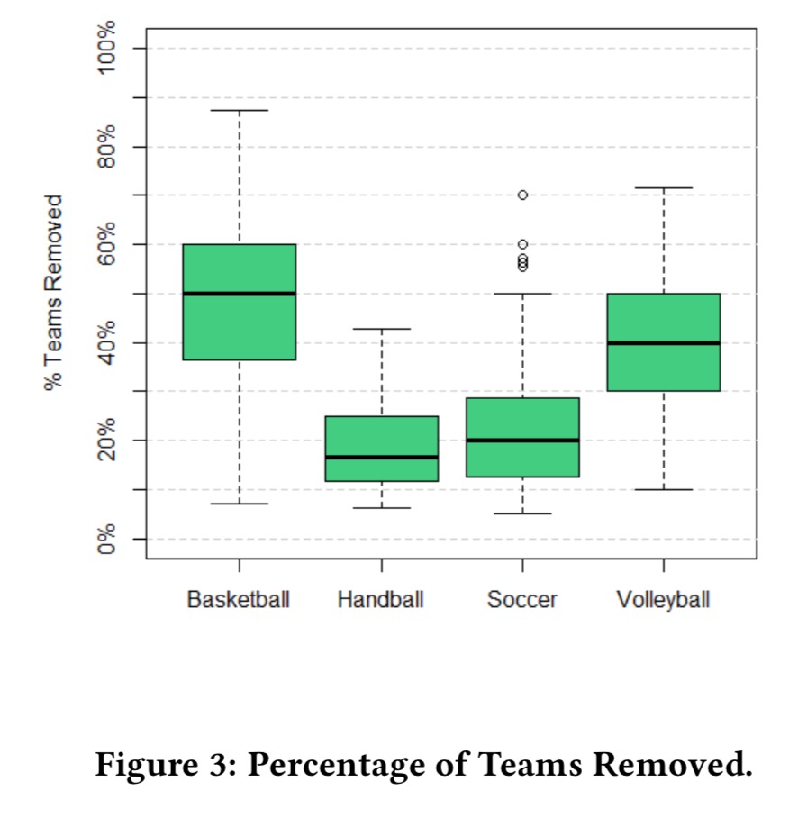
We saw the EPL example earlier. For the Spanish Primera Division (soccer) the average number of teams you need to remove is 3.2, which included Real Madrid and Barcelona for 9 out of the 10 seasons studied.
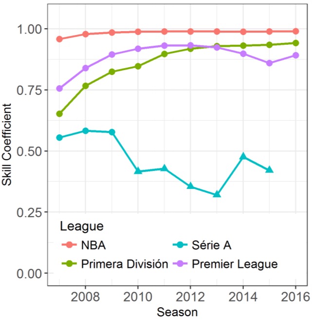
Looking at
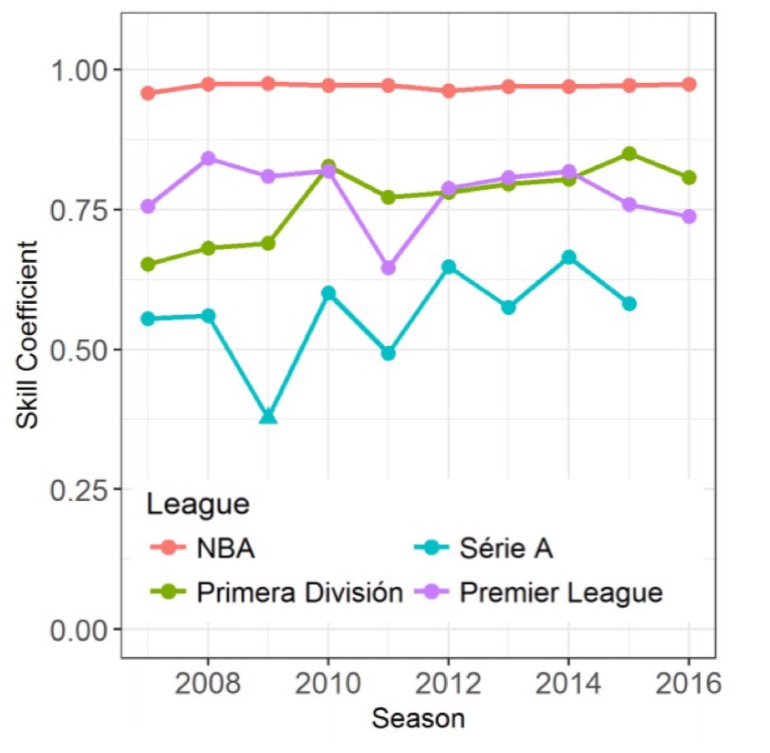
If we accumulate matches over all seasons in the dataset as if it where one long tournament we can see that for NBA, Serie A, and Primera Division the relative skills of teams are stable over the years, whereas in the Brazilian soccer league teams are more similar to each other in the long term.
A model of skills for NBA
What are the most important factors to explain the difference skills the teams show in a tournament?
The authors create a general Bayesian model based on Bradley-Terry that ends up looking like this:
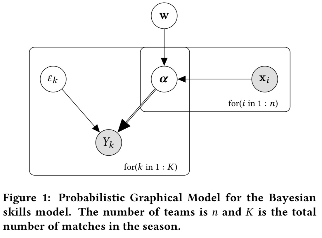
The skills coefficient for team 


For the NBA, considering matches during the regular season (and not the playoffs), the authors fit a Bayesian model with features in 
- A binary indicator indicating East conference or West conferences (the 30 teams are divided into two conferences)
- The average salary of the top five players
- The average Player Efficiency Rating (PER) in the last year
- Team volatility – how much a team changes its players between seasons
- Roster aggregate coherence – measuring the strength of the relationship between players (how long they have played together)
- Roster size – the number of players
(They tried several variations of features, these are the ones found to work the best). The following chart shows the correlation between team skills estimated by the model, and the number of games won during the regular season.
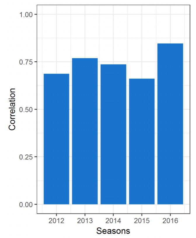
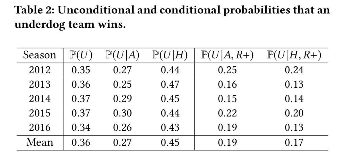
Table 2 (below) shows an important result. Based on the estimated skills
for each match, we are able to identify which team is the more skilled. Hence… we can estimate the probability that the underdog wins. It is stable over the seasons and approximately equal to 0.36. This is the component of luck in the NBA outcomes.
This turns out to be 0.45 when playing at home, and 0.27 when playing away. (The right-hand columns in the following table show what happens when you remove the top few most skilled teams from the equation).
In conclusion
After all this analysis, there’s a line in the conclusions that comes straight from the Ministry of the Bleeding Obvious: “Looking at the most relevant features, our results suggest a management strategy to maximize the formation of teams with high skills, the controllable aspect of team performance.” Well, duh!
Sports outcomes are a mix of skills and good and bad luck. This mix is responsible for a large part of the sports appeal…. The final message of our paper is that sometimes the culprit is luck, about 35% of the time in NBA. It is hard to beat luck in sports. This makes the joy and cheer of crowds [sic].
