Neural architecture search with reinforcement learning Zoph & Le, ICLR’17
Earlier this year we looked at ‘Large scale evolution of image classifiers‘ which used an evolutionary algorithm to guide a search for the best network architectures. In today’s paper, Zoph & Le also demonstrate that learning network architectures (and also in their case recurrent cell designs) can be stunningly effective. Stunningly effective as in very close to the state of the art on the CIFAR-10 dataset (and 0.09% better and 1.05x faster than the previous state of the art using a similar architectural scheme), and exceeding the current state-of-the-art on Penn Treebank, having composed a novel recurrent cell that outperforms the widely-used LSTM cell!
Not that long ago architectures were comparatively straightforward, and a lot of effort went into feature design. At that time we might have said, “although it has become easier, designing features still requires a lot of expert knowledge and takes ample time.” As we learned to learn features this ceased to be the case and, a paradigm shift from feature designing to architecture designing took place.
Although it has become easier, designing architectures still requires a lot of expert knowledge and takes ample time.
Are now we at the very beginning of a paradigm shift from architecture design to architecture learning? If you’ve got the computational budget (about 15,000x more expensive in terms of compute!), these early results suggest you can get world class results. What kind of budget do you need to get world class deep learning experts working on your problem? And will the search time (and hence cost) come down as we get smarter at searching for architectures? How about a Bayesian Optimisation approach for example?
Here’s Neural Architecture Search in a nutshell:
Our work is based on the observation that the structure and connectivity of a neural network can be typically specified by a variable-length string. It is therefore possible to use a recurrent network – the controller – to generate such a string. Training the network specified by the string – the “child network” – on the real data will result in an accuracy on a validation set. Using this accuracy as the reward signal, we can compute the policy gradient to update the controller. As a result, in the next iteration, the controller will give higher probabilities to architectures that receive high accuracies. In other words, the controller will learn to improve its search over time.
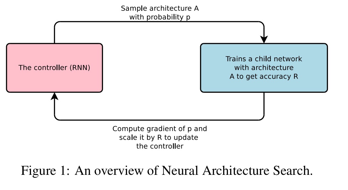
Let’s look in turn at how Neural Architecture Search generates network architectures, how it trains the controller, and how it speeds up training through parallel evaluation of multiple architectures in mini-batches.
Generating network architectures
Let’s begin by looking at how we can generate networks with only convolutional layers, and then build up to more sophisticated architectures. The controller that generates networks is implemented as a recurrent neural network.
Convolutional layers
Let’s suppose we would like to predict feedforward neural networks with only convolutional layers, we can use the controller to generate their hyperparameters as a sequence of tokens:
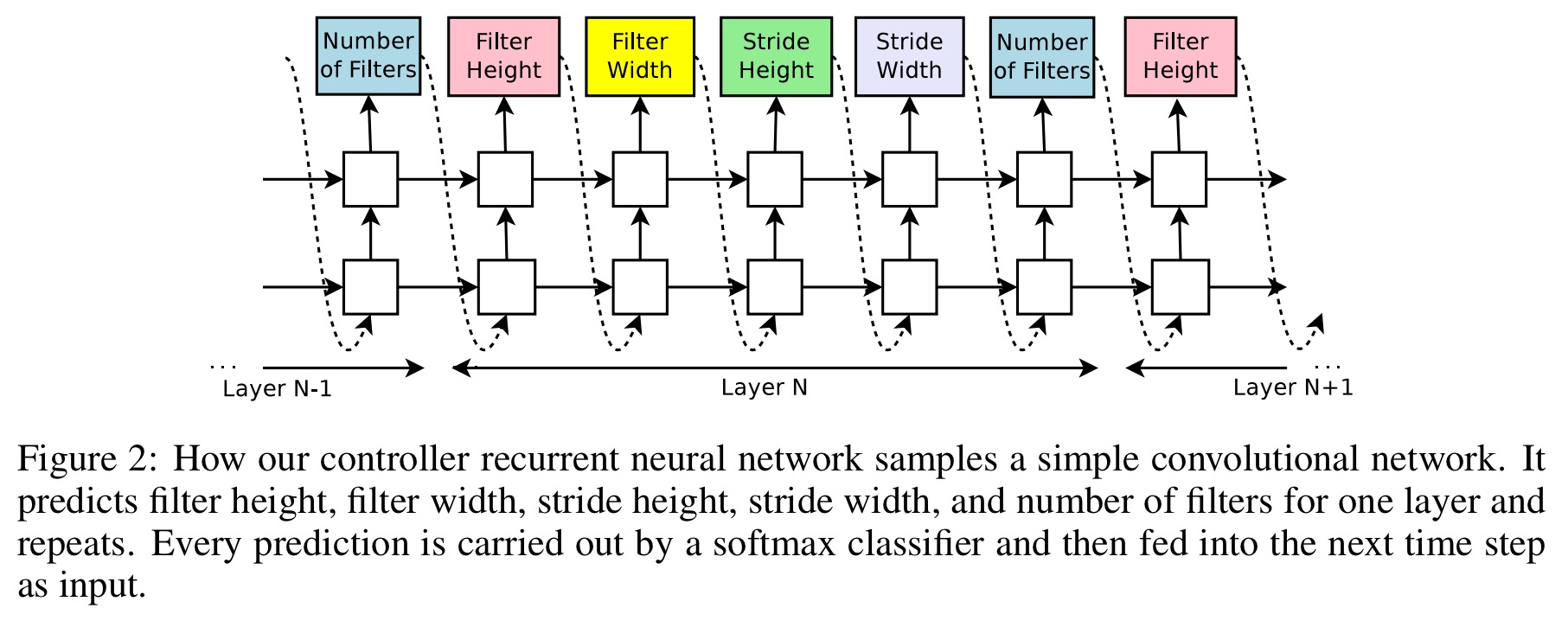
The number of layers in the generated architectures is controlled, and increases as training (of the controller) progresses.
Skip layers, pooling etc..
A set-selection type attention mechanism is used to predict skip connections.
At layer N, we add an anchor point which has N-1 content-based sigmoids to indicate the previous layers that need to be connected. Each sigmoid is a function of the current hidden state of the controller and the previous hidden states of the previous N-1 anchor points.
The controller samples from the sigmoids to decide what previous layers to be used as inputs to the current layer.
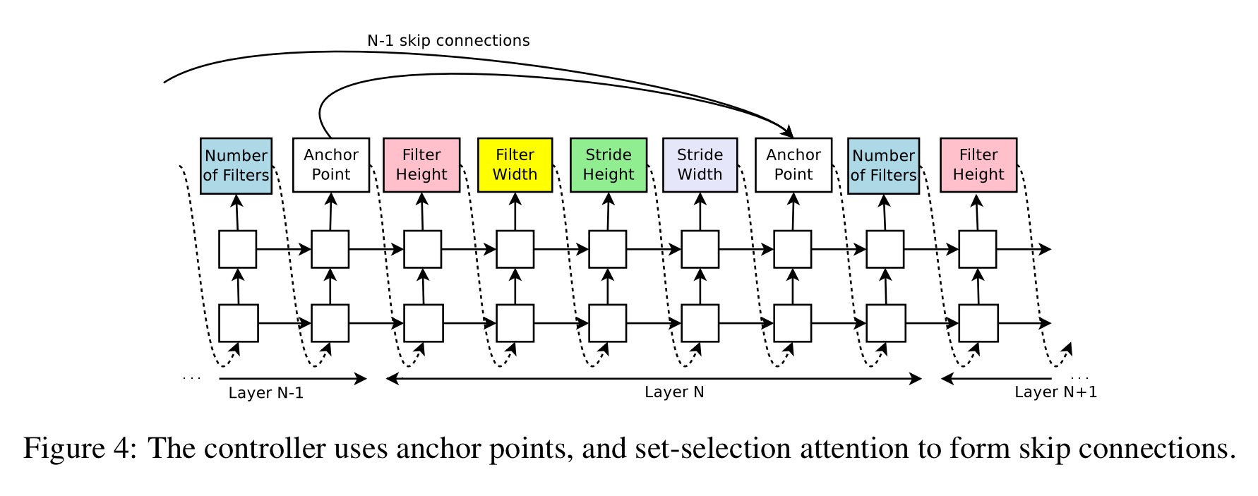
We can go further than just skip layers too:
It is possible to add learning rate as one of the predictions. Additionally, it is also possible to predict pooling, local contrast normalization, and batchnorm in the architectures. To be able to add more types of layers, we need to add an additional step in the controller RNN to predict the layer type, then other hyperparameters associated with it.
Recurrent cells
This is my favourite part! The controller is also set up to be able to generate novel recurrent cell designs.
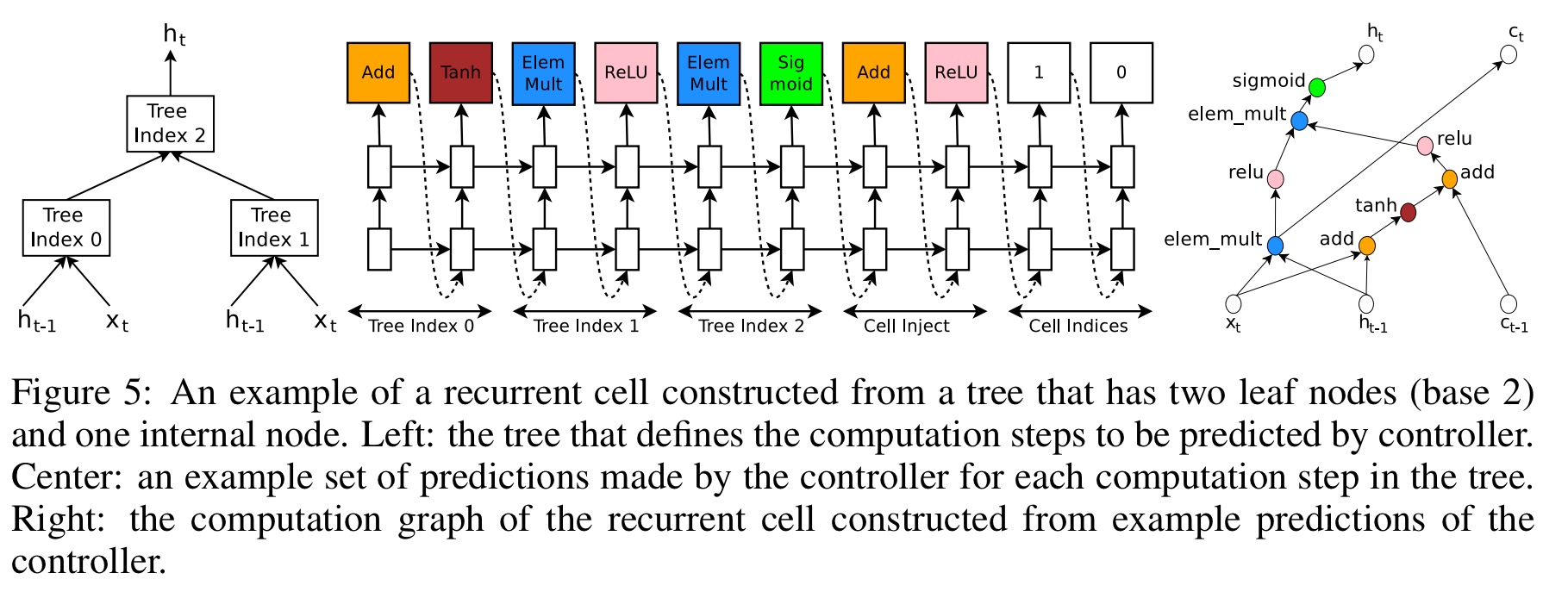
The computations for basic RNN and LSTM cells can be generalized as a tree of steps that take
and
as inputs and produce
as the final output. The controller RNN needs to label each node in the tree with a combination method (addition, elementwise multiplication, etc.) and an activation function (tanh, sigmoid, etc.) to merge two inputs and produce one output.
Two outputs are fed as inputs to the next node in the tree. There are also cell variables and
to represent the memory states. The controller RNN predicts what nodes in the tree to connect these too.
Training the controller
Once the controller RNN finishes generating an architecture, a neural network with this architecture is built and trained. At convergence, the accuracy of the network on a held-out validation set is recorded. The parameters of the controller RNN,
are then optimized to maximize the expected validation accuracy of the proposed architectures.
If we view the list of tokens predicted by the controller as a list of actions to design an architecture for a child network, then we can cast training as a reinforcement learning problem. The accuracy R that a trained child achieves is used as the reward signal to train the controller. The controller seeks to maximise the expected value of the reward. Since the reward signal is non-differentiable, a policy gradient method is used to update – in this case the REINFORCE rule (Williams 1992).
The update is given by

Where m is the number of different architectures that the controller samples in one batch and T is the number of hyperparameters the controller must predict to design an architecture. b is a baseline function (exponential moving average of the previous architecture accuracies) employed to reduce variance.
Accelerating training
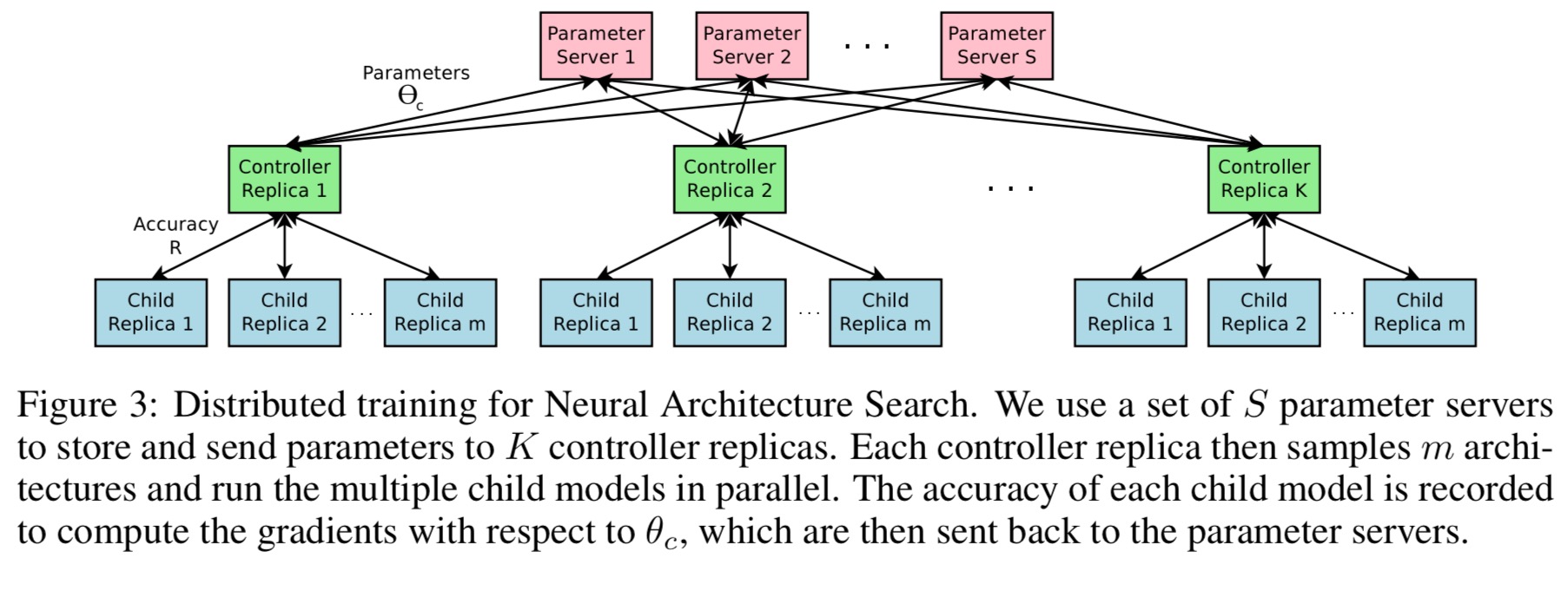
As training a child network can take hours, we use distributed training and asynchronous parameter updates in order to speed up the learning process of the controller.
A parameter server of S shards stores shared parameters for K controller replicas. Each replica samples m different child architectures that are trained in parallel. Weights are updates across all controller replicas at the end of each batch.
Experiments with CIFAR-10
Our search space consists of convolutional architectures, with rectified linear units as non-linearities, batch normalization, and skip connections between layers… The controller RNN is a two-layer LSTM with 35 hidden units on each layer. It is trained with the ADAM optimizer with a learning rate of 0.0006.
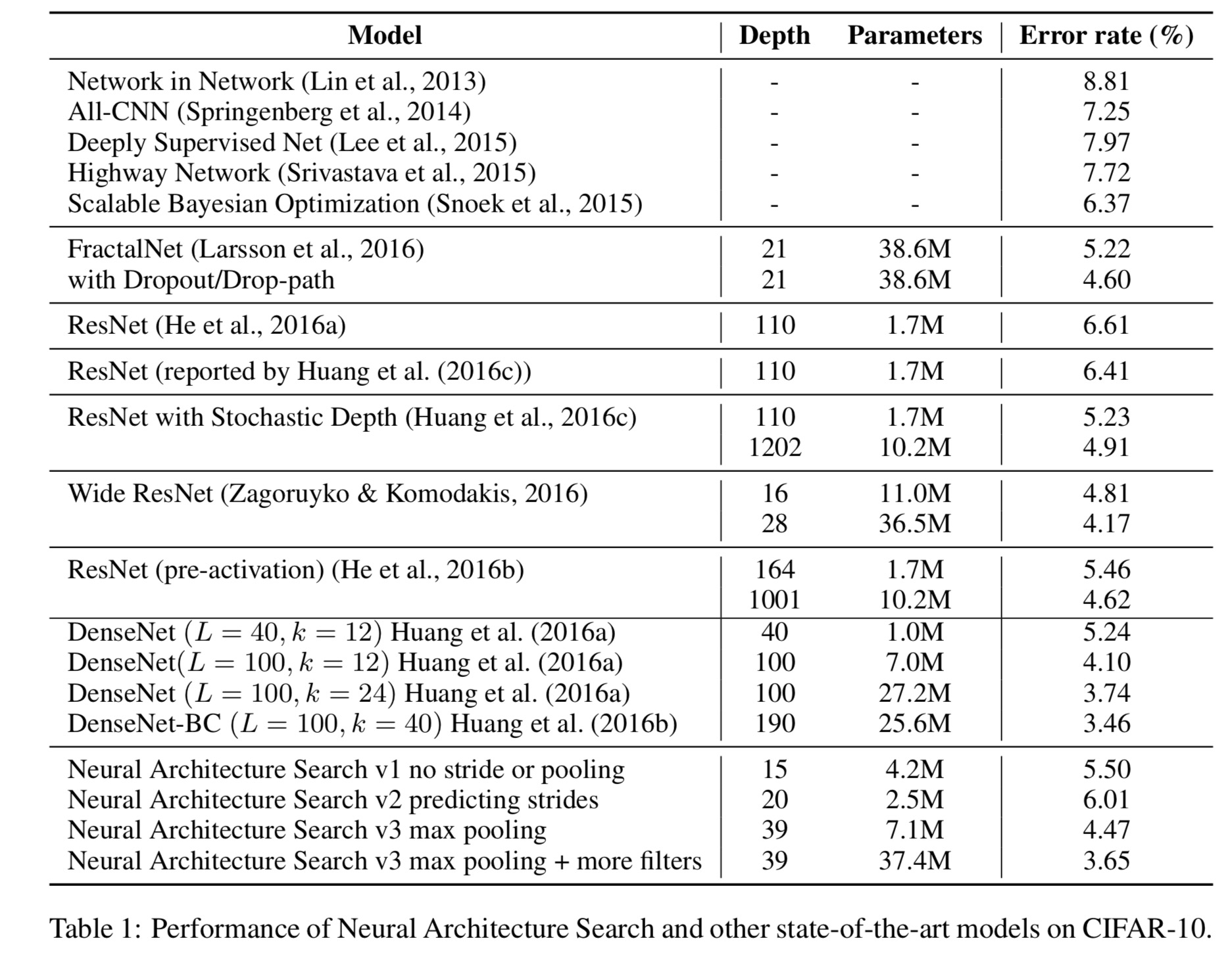
Each child model is trained for 50 epochs, with the reward function set to the validation accuracy of the last five epochs, cubed. After exploring 12,800 architectures, the best performing architecture is then run to convergence. “As can be seen from the table, Neural Architecture Search can design several promising architectures that perform as well as some of the best models on this dataset.”
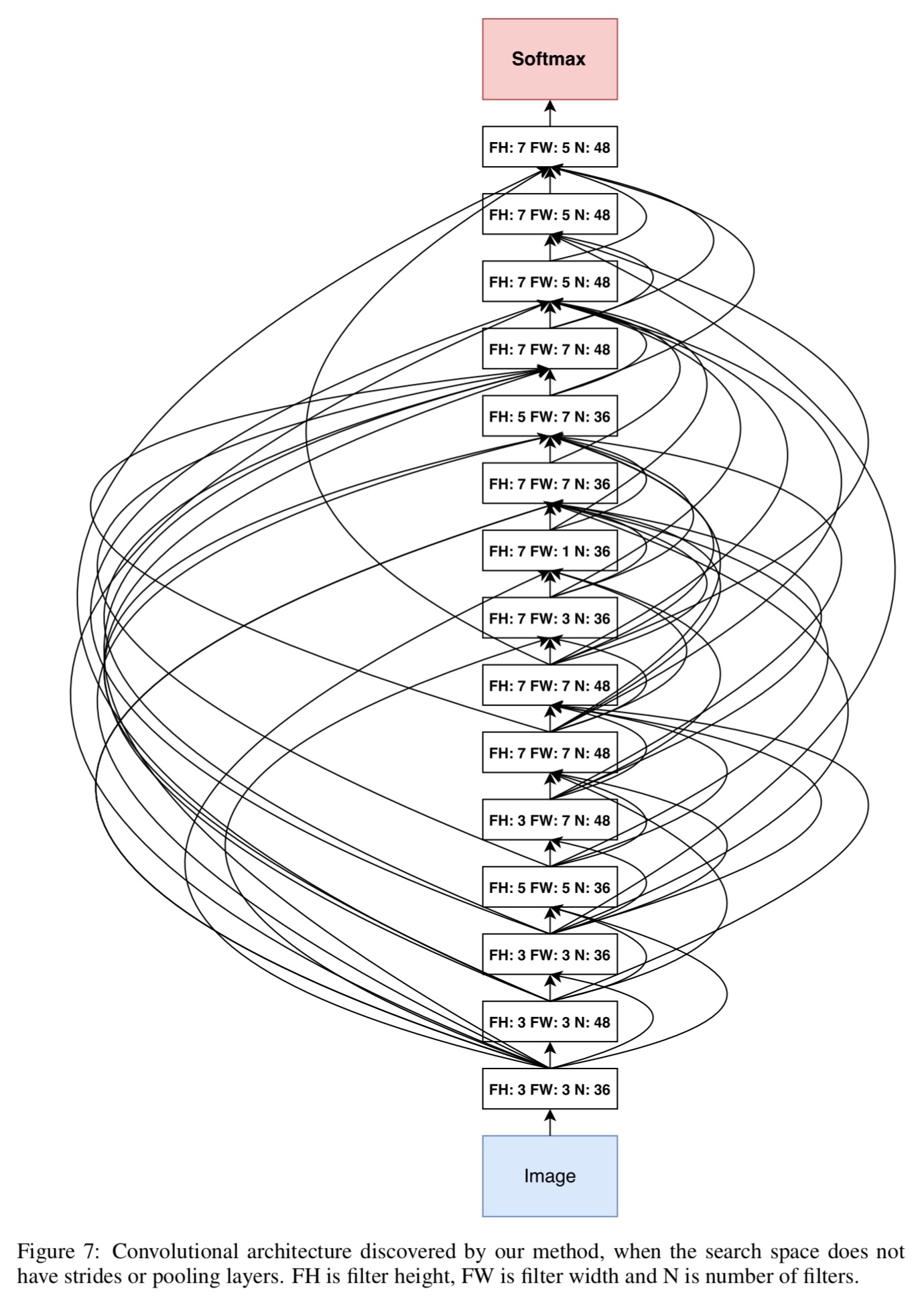
The learned “Neural Architecture Search v1” network from the above table looks like this:
Experiments with Penn Treebank
The controller RNN predicts a combination method and an activation function for each node in the tree. Training is done with 400 networks being trained across 400 CPUs at any one point in time. Parameter updates to the parameter server are made once 10 gradients have been accumulated from replicas. Each child model is trained for 35 epochs.
After the controller RNN is done training, we take the best RNN cell according to the lowest validation perplexity and then run a grid search over learning rate, weight initialization, dropout rates, and decay epoch. The best cell found was then run with three different configurations and sizes to increase its capacity.
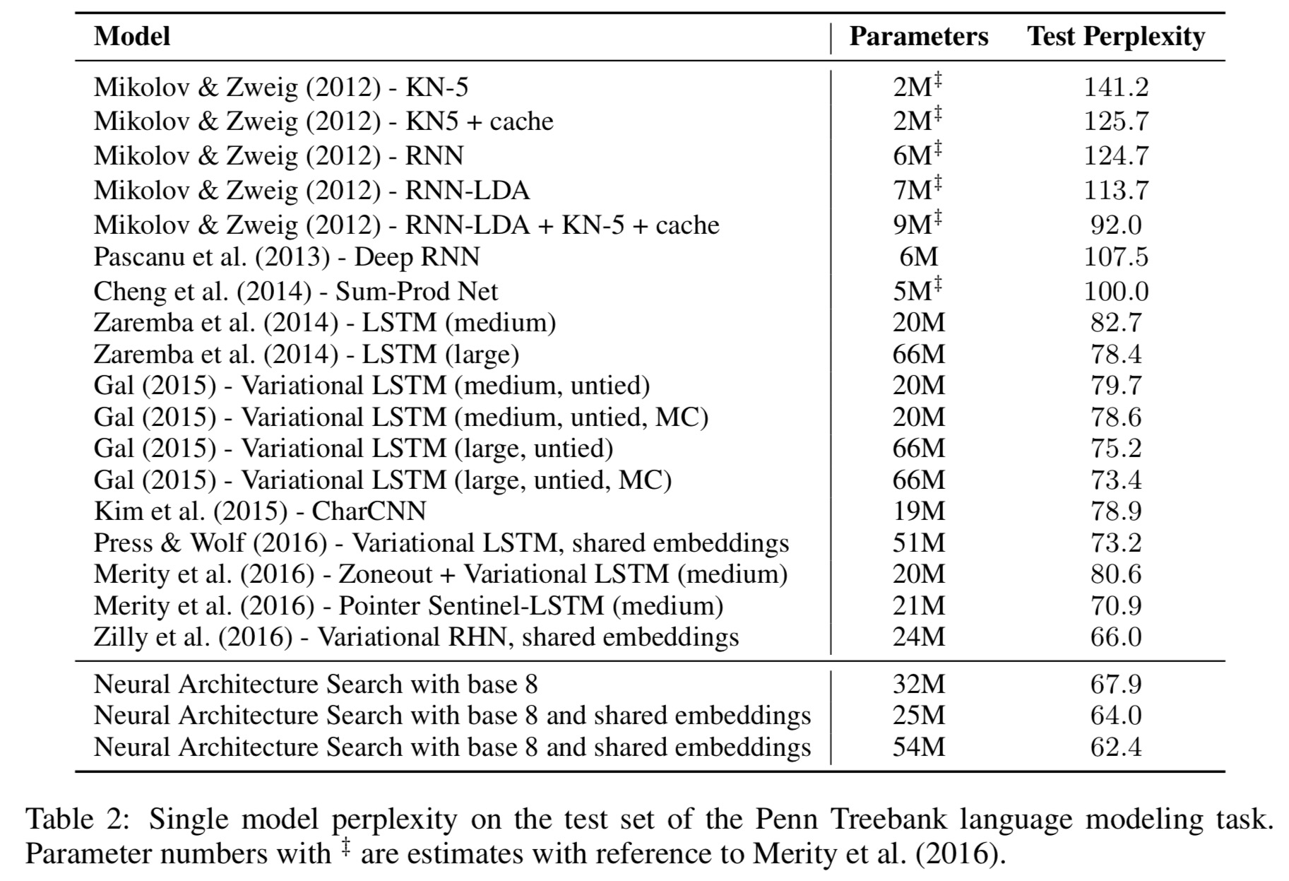
The models found outperform other state-of-the-art models on this dataset. “Not only is our cell better, the model that achieves 64 perplexity is also more than two times faster because the previous best network requires running a cell 10 times per time step.”
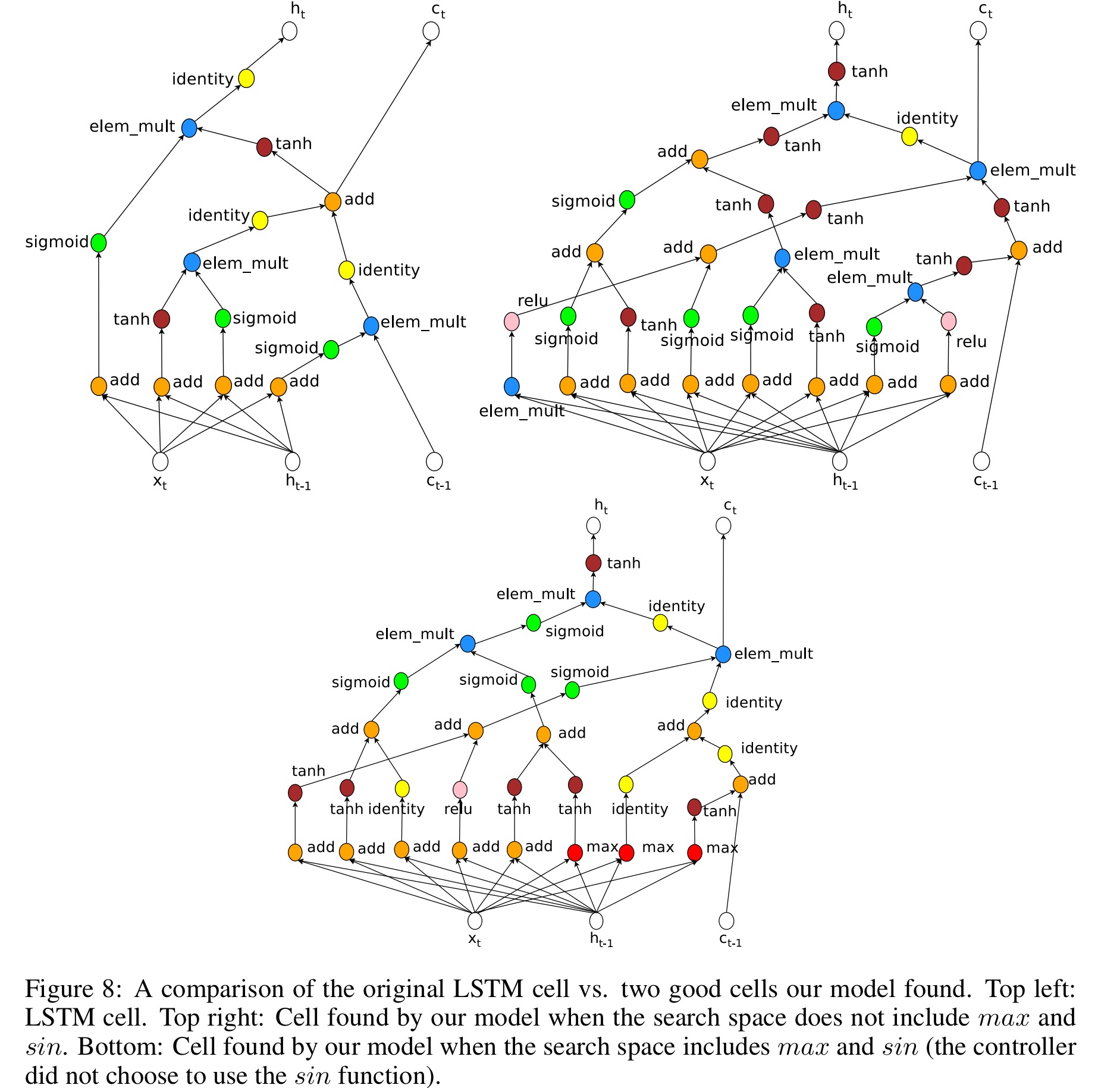
The newly discovered cell is visualized [below]. The visualization reveals that the new cell has many similarities to the LSTM cell in the first few steps, suchas it likes to compute
several times and send them to different components in the cell.
OK, but is it really better than random search
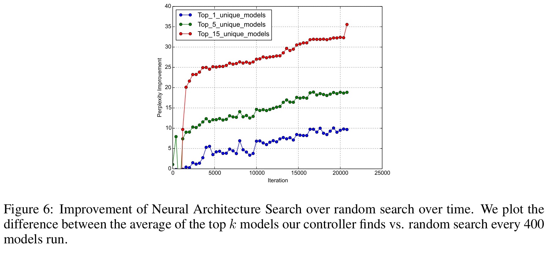
Checking performance against random search is an important sanity check. The best model found using the policy gradient approach in this paper is better than the best model found using random search, and the average of the top n models for several values of n is also found to be better.
It worth mentioning that resource usage is enormous – https://news.ycombinator.com/item?id=13440758
Yes indeed! I do call that out in the fourth paragraph – somewhere around 15,000x more expensive!!!
Great write up, as always! Glad you mentioned the potential 15000x cost increase!
The idea sounds *so* cool, but I worry that some models tend to perform initially good but top out fast, while other models take more iterations to train but achieve higher maximum validation accuracy. –> That means that for your controller to be able to evaluate each child’s R (accuracy) value, the child will need to have been (I mean, ideally…) quite fully trained (e.g. the 50 epochs they used). This issue is a problem for human researchers too, but the resulting cost effect isn’t so huge.
When dealing with models that train of millions of observations, the sheer amount of $$$ to do something like this using AWS sounds prohibitive (unless you’re, like, Google). 15000x is so high when x = 20% of a team’s budget :O.
We did some work on using BO for deep structure optimizxation. Take a look at this paper:
Ramachandram, D., Lisicki, M., Shields, T., Amer, M. and Taylor, G.W., “Structure optimization for deep multimodal fusion networks using graph-induced kernels”, Proc. of 25th European Symposium on Artificial Neural Networks, Computational Intelligence and Machine Learning (ESANN 2017), Apr 26-28, Bruges, Belgium.
Questions:
1. What is the input to the Controller RNN at each time-step?
2. What is the embedding that is passed between layers, mentioned in the presentation(http://rll.berkeley.edu/deeprlcourse/docs/quoc_barret.pdf) on slide 7?
I have the same question, did you figure it out?