Large-scale evolution of image classifiers Real et al., 2017

I’m sure you noticed the bewildering array of network architectures in use when we looked at some of the top convolution neural network papers of the last few years last week (Part 1, Part2, Part 3). With sufficient training data, these networks can achieve amazing feats, but how do you find the best network architecture for your problem in the first place?

Discovering neural network architectures… remains a laborious task. Even within the specific problem of image classification, the state of the the art was attained through many years of focused investigation by hundreds of researchers.

If you’re an AI researcher and you come up against a difficult problem where it’s hard to encode the best rules (or features) by hand, what do you do? Get the machine to learn them for you of course! If what you want to learn is a function, and you can optimise it through back propagation, then a network is a good solution (see e.g. ‘Network in Network‘, or ‘Learning to learn by gradient descent by gradient descent‘). If what you want to learn is a policy that plays out over some number of time steps then reinforcement learning would be a good bet. But what if you wanted to learn a good network architecture? For that the authors turned to a technique from the classical AI toolbox, evolutionary algorithms.

As you may recall, evolutionary algorithms start out with an initial population, assess the suitability of population members for the task in hand using some kind of fitness function, and then generate a new population for the next iteration by mutations and combinations of the fittest members. So we know that we’re going to start out with some population of initial model architectures (say, 1000 of them), define a fitness function based on how well they perform when trained, and come up with a set of appropriate mutation operations over model architectures. That’s the big picture, and there’s just one more trick from the deep learning toolbox that we need to bring to bear: brute force! If in doubt, overwhelm the problem with bigger models, more data, or in this case, more computation:

We used slightly-modified known evolutionary algorithms and scaled up the computation to unprecedented levels, as far as we know. This, together with a set of novel and intuitive mutation operators, allowed us to reach competitive accuracies on the CIFAR-10 dataset. This dataset was chosen because it requires large networks to reach high accuracies, thus presenting a computational challenge.

The initial population consists of very simple (and very poorly performing) linear models, and the end result is a fully trained neural network with no post-processing required. Here’s where the evolved models stand in the league table:

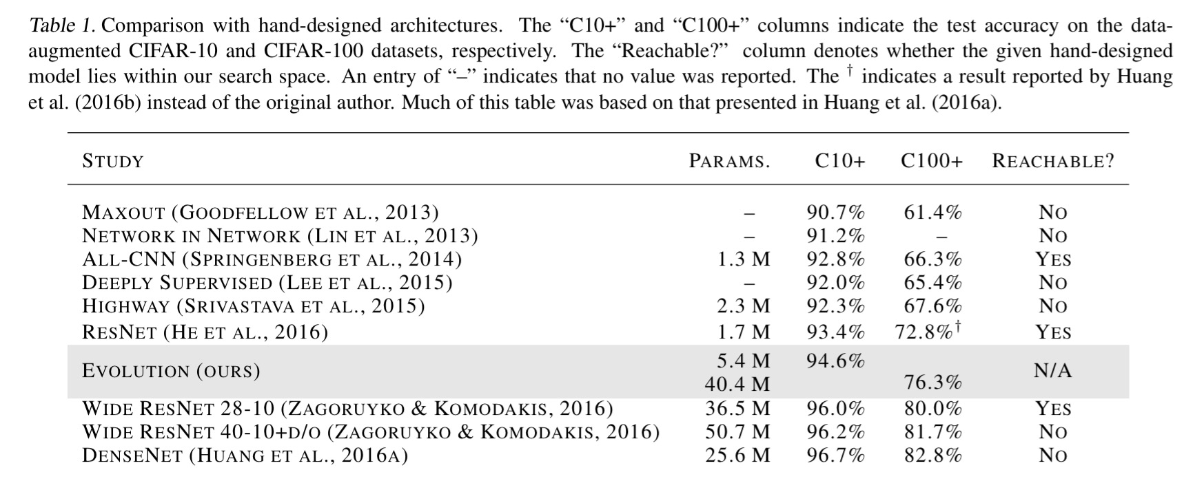
That’s a pretty amazing result when you think about it. Really top-notch AI researchers are in very short supply, but computation is much more readily available on the open market. ‘Evolution’ evolved an architecture, with no human guidance, that beats some of our best models from the last few years.

Let’s take a closer look at the details of the evolutionary algorithm, and then we’ll come back and dig deeper into the evaluation results.

Evolving models

We start with a population of 1000 very simple linear regression models, and then use tournament selection. During each evolutionary step, a worker process (250 of them running in parallel) chooses two individuals at random and compares their fitness. The worst of the pair is removed from the population, and the better model is chosen as a parent to help create the next generation. A mutation is applied to the parent to create a child. The worker then trains the child, evaluates it on the validation set, and puts it back into the population.

Using this strategy to search large spaces of complex image models requires considerable computation. To achieve scale, we developed a massively-parallel, lock-free infrastructure. Many workers operate asynchronously on different computers. They do not communicate directly with each other. Instead, they use a shared file-system, where the population is stored.

Training and validation takes place on the CIFAR-10 dataset consisting of 50,000 training examples and 10,000 test examples, all labeled with 1 of 10 common object classes. Each training runs for 25,600 steps – brief enough so that each individual can be trained somewhere between a few seconds and a few hours, depending on the model size. After training, a single evaluation on the validation set provides the accuracy to use as the model’s fitness.

We need architectures that are trained to completion within an evolutionary experiment… [but] 25,600 steps are not enough to fully train each individual. Training a large enough model to completion is prohibitively slow for evolution. To resolve this dilemma, we allow the children to inherit the parents’ weights whenever possible.

The final piece of the puzzle then, is the encoding of model architectures, and the mutation operations defined over them. A model architecture is encoded as a graph (its DNA). Vertices are tensors or activations (either batch normalisation with ReLUs, or simple linear units). Edges in the graph are identity connections (for skipping) or convolutions.

When multiple edges are incident on a vertex, their spatial scales or numbers of channels may not coincide. However, the vertex must have a single size and number of channels for its activations. The inconsistent inputs must be resolved. Resolution is done by choosing one of the incoming edges as the primary one. We pick this primary edge to be the one that is not a skip connection.

Activation functions are similarly reshaped (using some combination of interpolation, truncation, and padding), and the learning rate is also encoded in the DNA.

When creating a child, a worker picks a mutation at random from the following set:

• Alter learning rate
• Identity (effectively gives the individual further training time in the next generation)
• Reset weights
• Insert convolution (at a random location in the ‘convolutional backbone’). Convolutions are 3×3 with strides of 1 or 2.
• Remove convolution
• Alter stride (powers of 2 only)
• Alter number of channels (of a random convolution)
• Filter size (horizontal or vertical at random, on a random convolution, odd values only)
• Insert one-to-one (adds a one-to-one / identity connection)
• Add skip (identity between random layers)
• Remove skip (removes a random skip)

Evaluation results

Here’s an example of an evolution experiment, with selected population members highlighted:

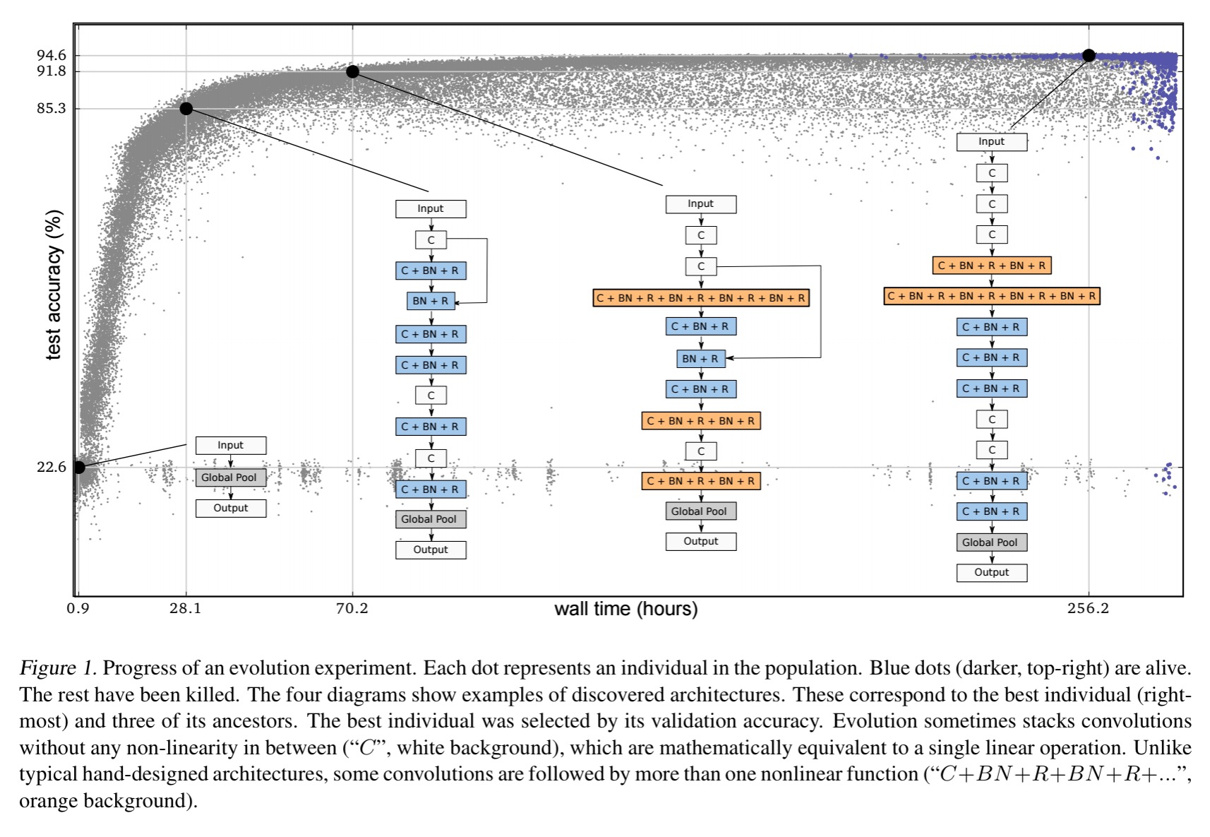
Five experiment runs are done, and although not all models reach the same accuracy, they get pretty close. It took 9 x 10¹⁹ FLOPs on average per experiment.

The following chart shows how accuracy improves over time during the experiments:

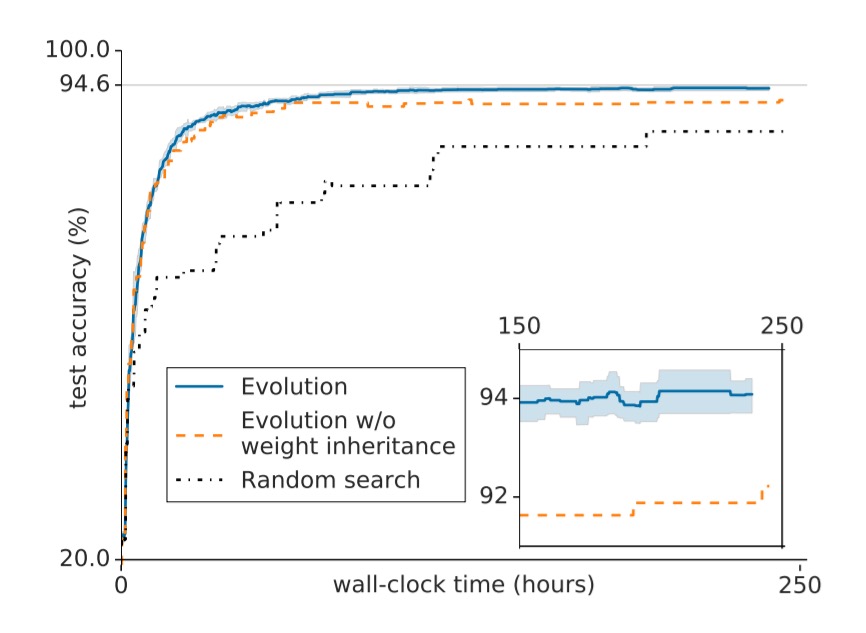
We observe that populations evolve until they plateau at some local optimum. The fitness (i.e. validation accuracy) value at this optimum varies between experiments (Above, inset). Since not all experiments reach the highest possible value, some populations are getting “trapped” at inferior local optima. This entrapment is affected by two important meta-parameters (i.e. parameters that are not optimized by the algorithm). These are the population size and the number of training steps per individual.

The larger the population size, the more thoroughly the space of models can be explored, which helps to reach better optima. More training time means that a model needs to undergo fewer identity mutations to reach a given level of training (remember that the end result of the evolution process is a fully trained model, not just a model architecture).

Two other approaches to escaping local optima are increasing the mutation rate, and resetting weights. When it looks like members of the population are trapped in poor local optima, the team tried applying 5 mutations instead of 1 for a few generations. During this period some population members escape the local optimum, and none get worse:

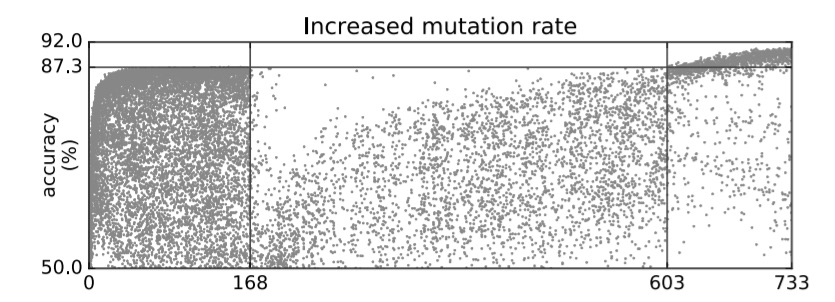
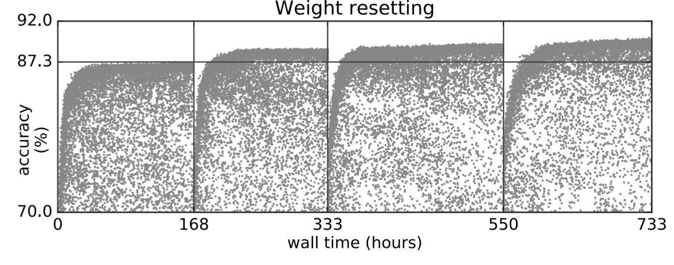
To avoid getting trapped by poorer architectures that just happened to have received more training (e.g. through the identity mutation), the team also tried experiments in which the weights are simultaneously reset across all population members when a plateau is reached. The populations suffer a temporary degradation (as to be expected), but ultimately reach a higher optima.