Today we’re pressing on with the top 100 awesome deep learning papers list, and the section on recurrent neural networks (RNNs). This contains only four papers (joy!), and even better we’ve covered two of them previously (Neural Turing Machines and Memory Networks, the links below are to the write-ups). That leaves up with only two papers to cover today, however the first paper does run to 43 pages and it’s a lot of fun so I’m glad to be able to devote a little more space to it.
- Generating sequences with recurrent neural networks, Graves 2013
- Conditional random fields as recurrent neural networks, Zheng and Jayasumana, 2015
- Neural Turing machines
- Memory networks
These papers are easier to understand with some background in RNNs and LSTMs. Christopher Olah has a wonderful post on “Understanding LSTM networks” which I highly recommend.
Generating sequences with recurrent neural networks
This paper explores the use of RNNs, in particular, LSTMs, for generating sequences. It looks at sequences over discrete domains (characters and words), generating synthetic wikipedia entries, and sequences over real-valued domains, generating handwriting samples. I especially like the moment where Graves demonstrates that the trained networks can be used to ‘clean up’ your handwriting, showing what a slightly neater / easier to read version of your handwriting could look like. We’ll get to that shortly…
RNNs can be trained for sequence generation by processing real data sequences one step at a time and predicting what comes next. Assuming the predictions are probabilistic, novel sequences can be generated from a trained network by iteratively sampling from the network’s output distribution, then feeding in the sample as input at the next step. In other words by making the network treat its inventions as if they were real, much like a person dreaming.
Using LSTMs effectively gives the network a longer memory, enabling it to look back further in history to formulate its predictions.
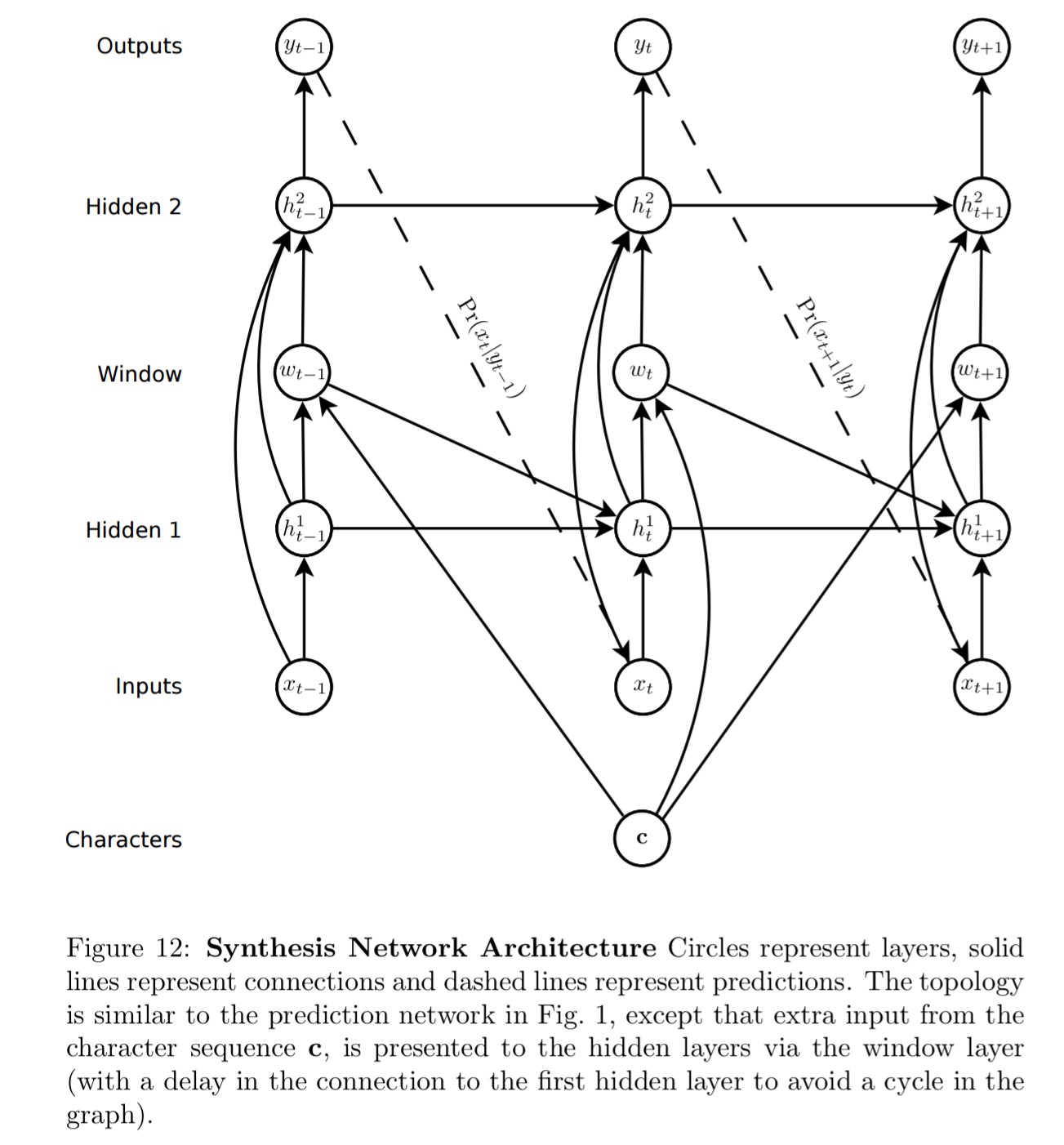
The basic RNN architecture used for all the models in the paper looks like this:
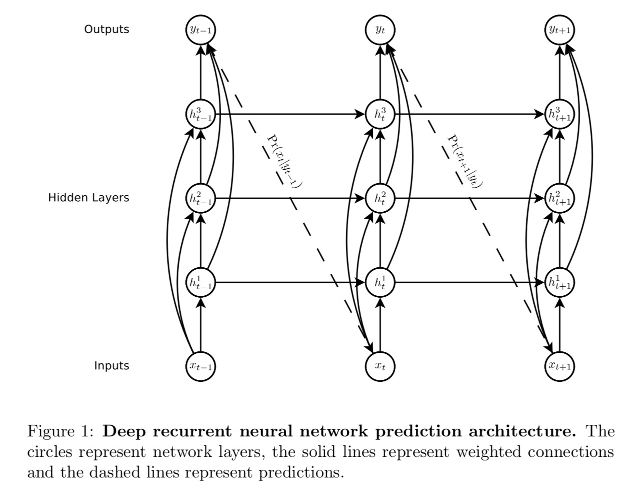
Note how each output vector is used to parameterise a predictive distribution
over the next possible inputs (the dashed lines in the above figure). Also note the use of ‘skip connections’ as we looked at in yesterday’s post.
The LSTM cells used in the network look like this:
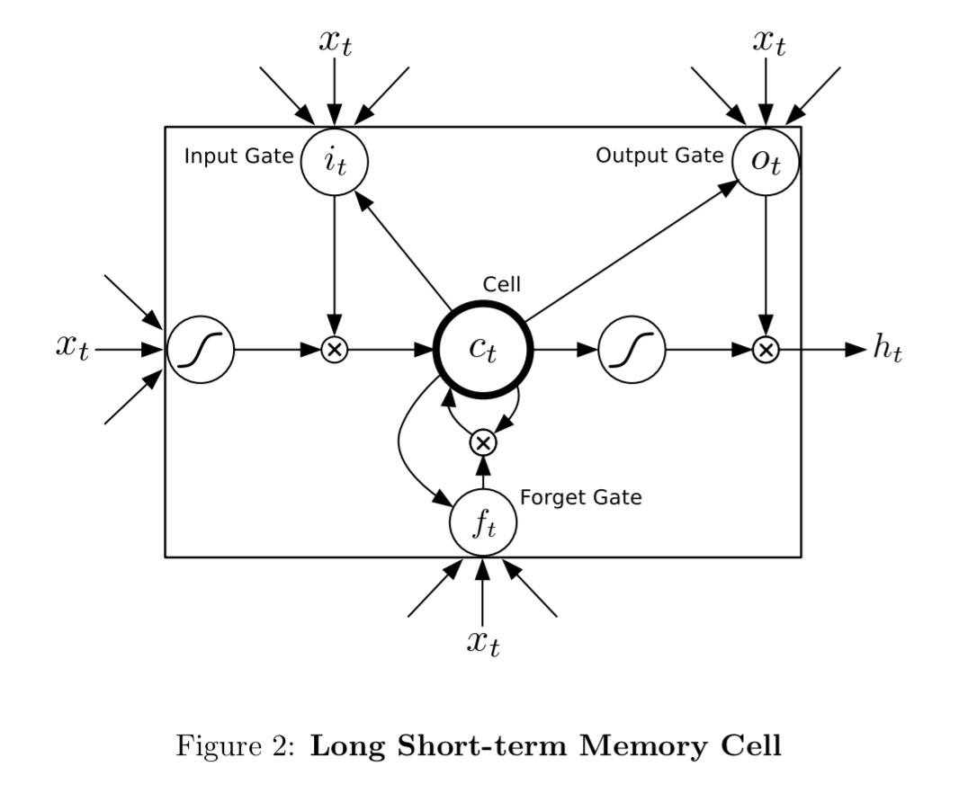
They are trained with the full gradient using backpropagation. To prevent the derivatives becoming too large, the derivative of the loss with respect to the inputs to the LSTM layers are clipped to lie within a predefined range.
Onto the experiments…
Text prediction
For text prediction we can either use sequences of words, or sequences of characters. With one-hot encodings, the number of different classes for words makes for very large input vectors (e.g. a vocabulary with 10’s of thousands of words of more). In contrast, the number of characters is much more limited. Also,
… predicting one character at a time is more interesting from the perspective of sequence generation, because it allows the network to invent novel words and strings. In general, the experiments in this paper aim to predict at the finest granularity found in the data, so as to maximise the generative flexibility of the network.
The Penn Treebank dataset is a selection of Wall Street Journal articles. It’s relatively small at just over a million words in total, but widely used as a language modelling benchmark. Both word and character level networks were trained on this corpus using a single hidden layer with 1000 LSTM units. Both networks are capable of overfitting the training data, so regularisation is applied. Two forms of regularisation were experimented with: weight noise applied at the start of each training sequence, and adaptive weight noise, where the variance of the noise is learned along with the weights.
The word-level RNN performed better than the character-based one, but the gap closes with regularisation (perplexity of 117 in the best word-based configuration, vs 122 for the best character-based configuration).
“Perplexity can be considered to be a measure of on average how many different equally most probable words can follow any given word. Lower perplexities represent better language models…” ([][] http://www1.icsi.berkeley.edu/Speech/docs/HTKBook3.2/node188_mn.html )
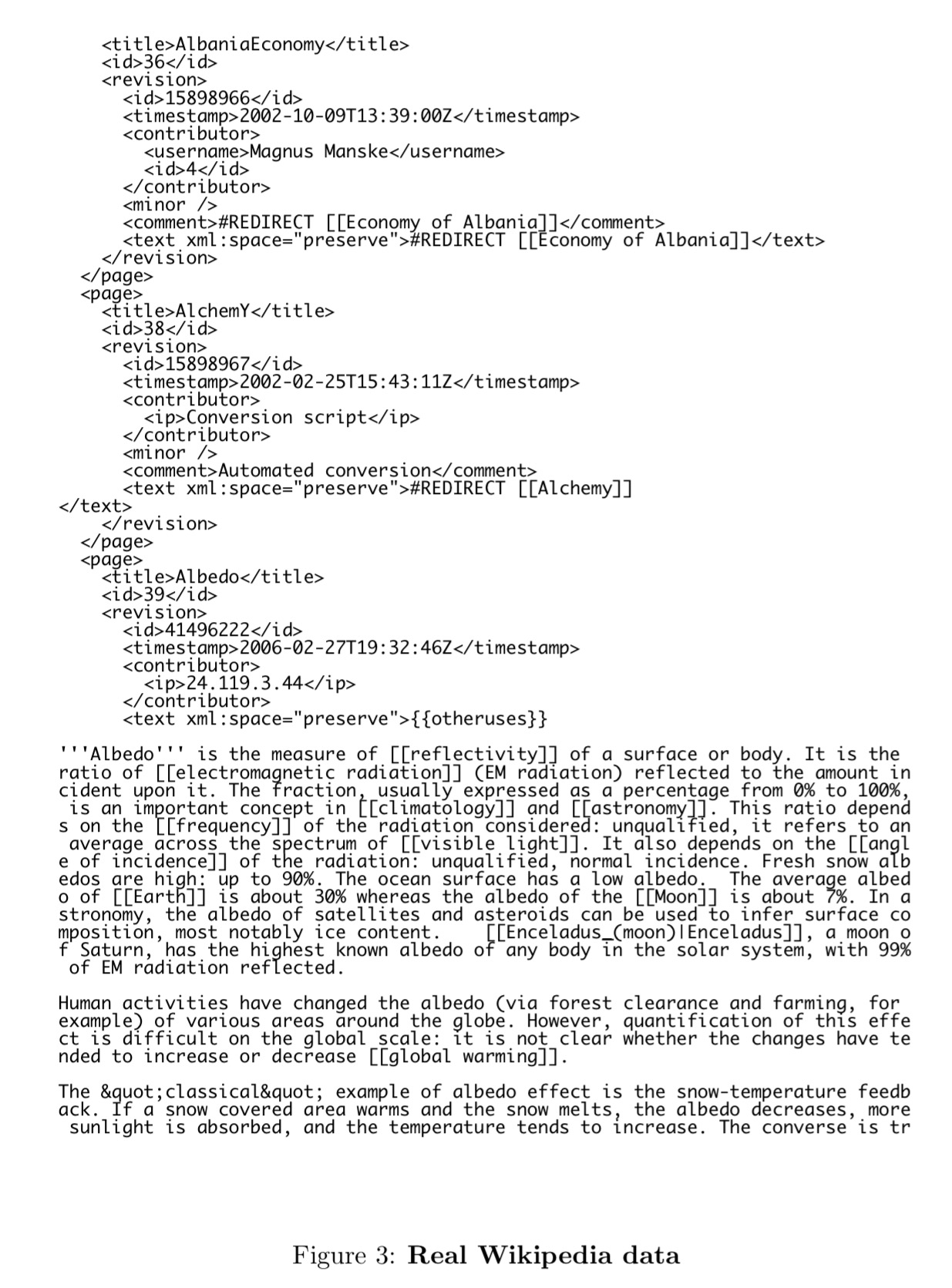
Much more interesting is a network that Graves trains on the first 96M bytes of the Wikipedia corpus (as of March 3rd 2006, captured for the Hutter prize competition). This has seven hidden layers of 700 LSTM cells each. This is an extract of the real Wikipedia data:
And here’s a sample generated by the network (for additional samples, see the full paper):
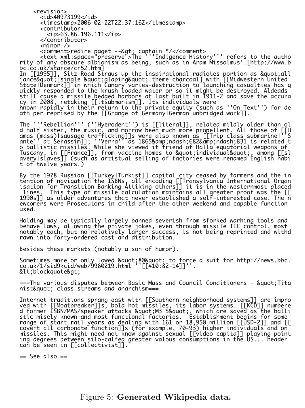
The sample shows that the network has learned a lot of structure from the data, at a wide range of different scales. Most obviously, it has learned a large vocabulary of dictionary words, along with a subword model that enables it to invent feasible-looking words and names: for example “Lochroom River”, “Mughal Ralvaldens”, “submandration”, “swalloped”. It has also learned basic punctuation, with commas, full stops and paragraph breaks occurring at roughly the right rhythm in the text blocks.
It can correctly open and close quotation marks and parentheses, indicating the models memory and these often span a distance that a short-range context cannot handle. Likewise, it can generate distinct large-scale regions such as XML headers, bullet-point lists, and article text.
Of course, the actual generated articles don’t make any sense to a human reader, it is just their structure that is mimicked. When we move onto handwriting though, the outputs do make a lot of sense to us…
Handwriting prediction
To test whether the prediction network could also be used to generate convincing real-valued sequences, we applied it to online handwriting data (online in this context means that the writing is recorded as a sequence of pen-tip locations, as opposed to offline handwriting, where only the page images are available). Online handwriting is an attractive choice for sequence generation due to its low dimensionality (two real numbers per data point) and ease of visualisation.
The dataset consists of handwritten lines on a smart whiteboard, with x,y co-ordinates and end-of-stroke markers (yes/no) captured at each time point. The main challenge was figuring out how to determine a predictive distribution for real-value inputs. The solution is to use mixture density neworks. Here the outputs of the network are used to parameterise a mixture distribution. Each output vector consists of the end of stroke probability e, along with a set of means, standard deviations, correlations, and mixture weights for the mixture components used to predict the x and y positions. See pages 20 and 21 for the detailed explanation.
Here are the mixture density outputs for predicted locations as the word under is written. The small blobs show accurate predictions while individual strokes are being written, and the large blobs show greater uncertainty at the end of strokes when the pen is lifted from the whiteboard.
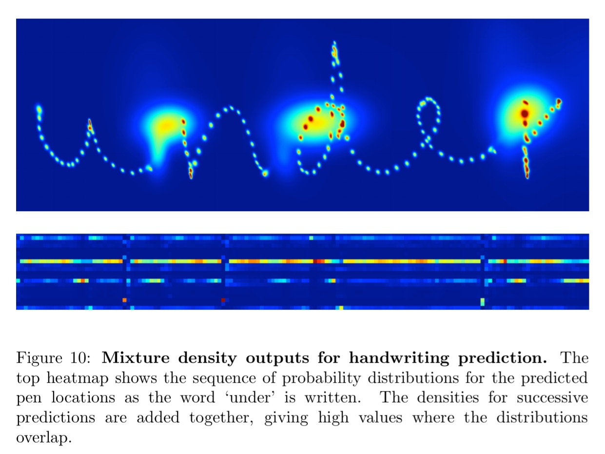
The best samples were generated by a network with three hidden layers of 400 LSTM cells each, and 20 mixture components to model the offsets. Here are some samples created by the network.
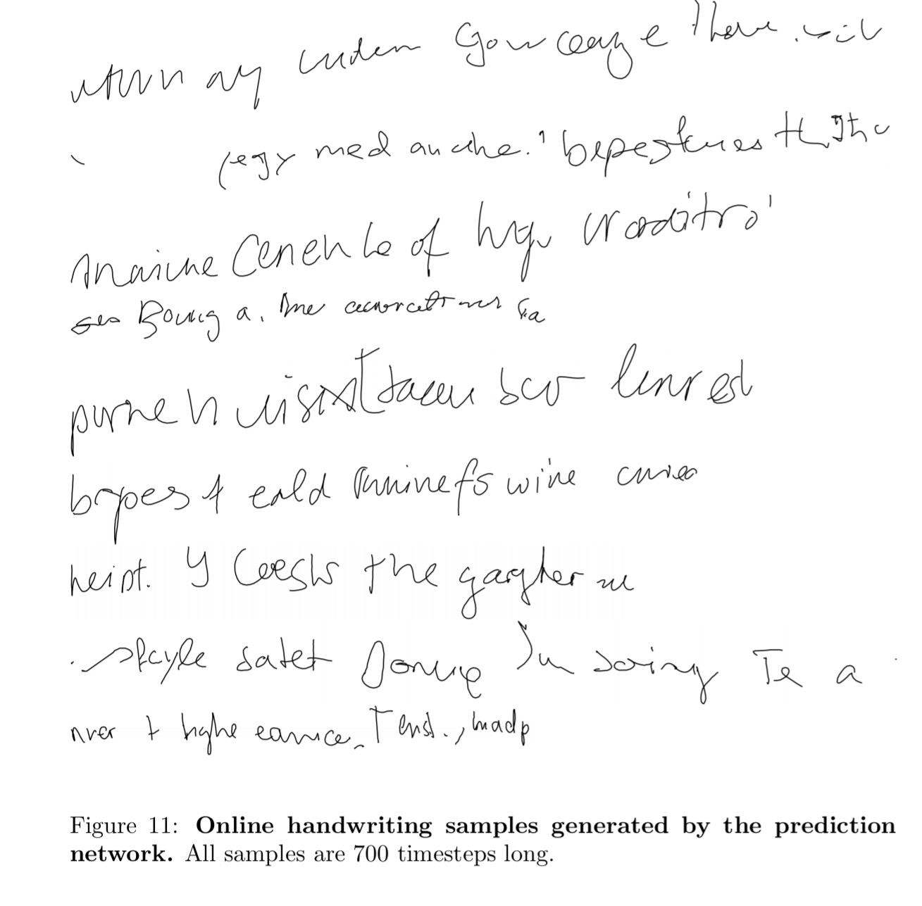
The network has clearly learned to model strokes, letters and even short words (especially common ones such as ‘of’ and ‘the’). It also appears to have learned a basic character level language models, since the words it invents (‘eald’, ‘bryoes’, ‘lenrest’) look somewhat plausible in English. Given that the average character occupies more than 25 timesteps, this again demonstrates the network’s ability to generate coherent long-range structures
Handwriting generation
Those samples do of course look like handwriting, but as with our Wikipedia example, the actual words are nonsense. Can we learn to generated handwriting for a given text? To meet this challenge a soft window is convolved with the text string and fed as an extra input to the prediction network.
The parameters of the window are output by the network at the same time as it makes the predictions, so that it dynamically determines an alignment between the text and the pen locations. Put simply, it learns to decide which character to write next.
The network learns how far to slide the text window at each step, rather than learning an absolute position. “Using offsets was essential to getting the network to align the text with the pen trace.”
And here are samples generated by the resulting network:
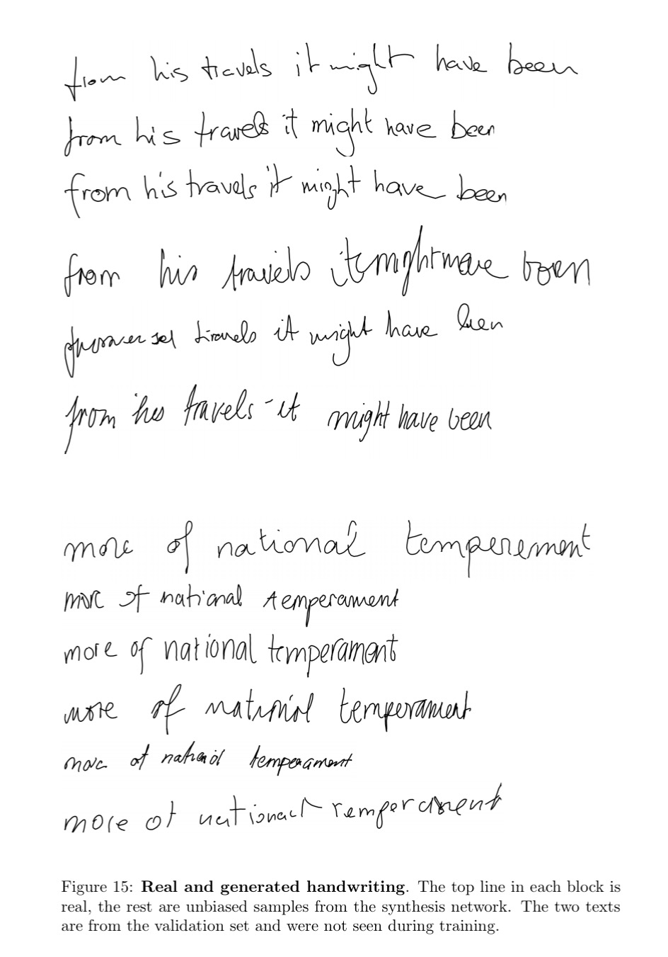
Pretty good!
Biased and primed sampling to control generation
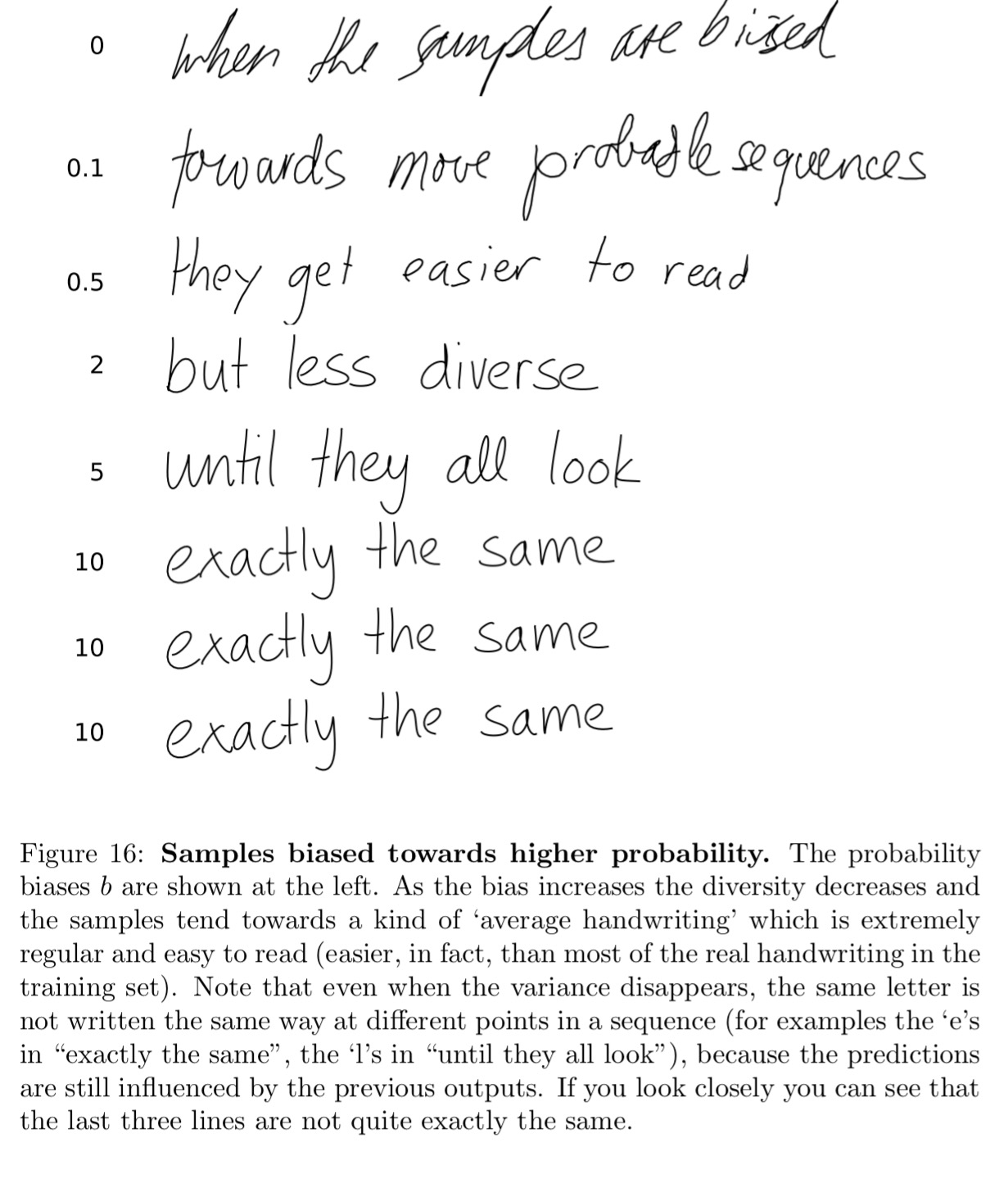
One problem with unbiased samples is that they tend to be difficult to read (partly because real handwriting is difficult to read, and partly because the network is an imperfect model). Intuitively, we would expect the network to give higher probability to good handwriting because it tends to be smoother and more predictable than bad handwriting. If this is true, we should aim to output more probable elements of Pr(x|c) if we want the samples to be easier to read. A principled search for high probability samples could lead to a difficult inference problem, as the probability of every output depends on all previous outputs. However a simple heuristic, where the sampler is biased towards more probable predictions at each step independently, generally gives good results.
As we increase the bias towards higher probability predictions, the handwriting gets neater and neater…
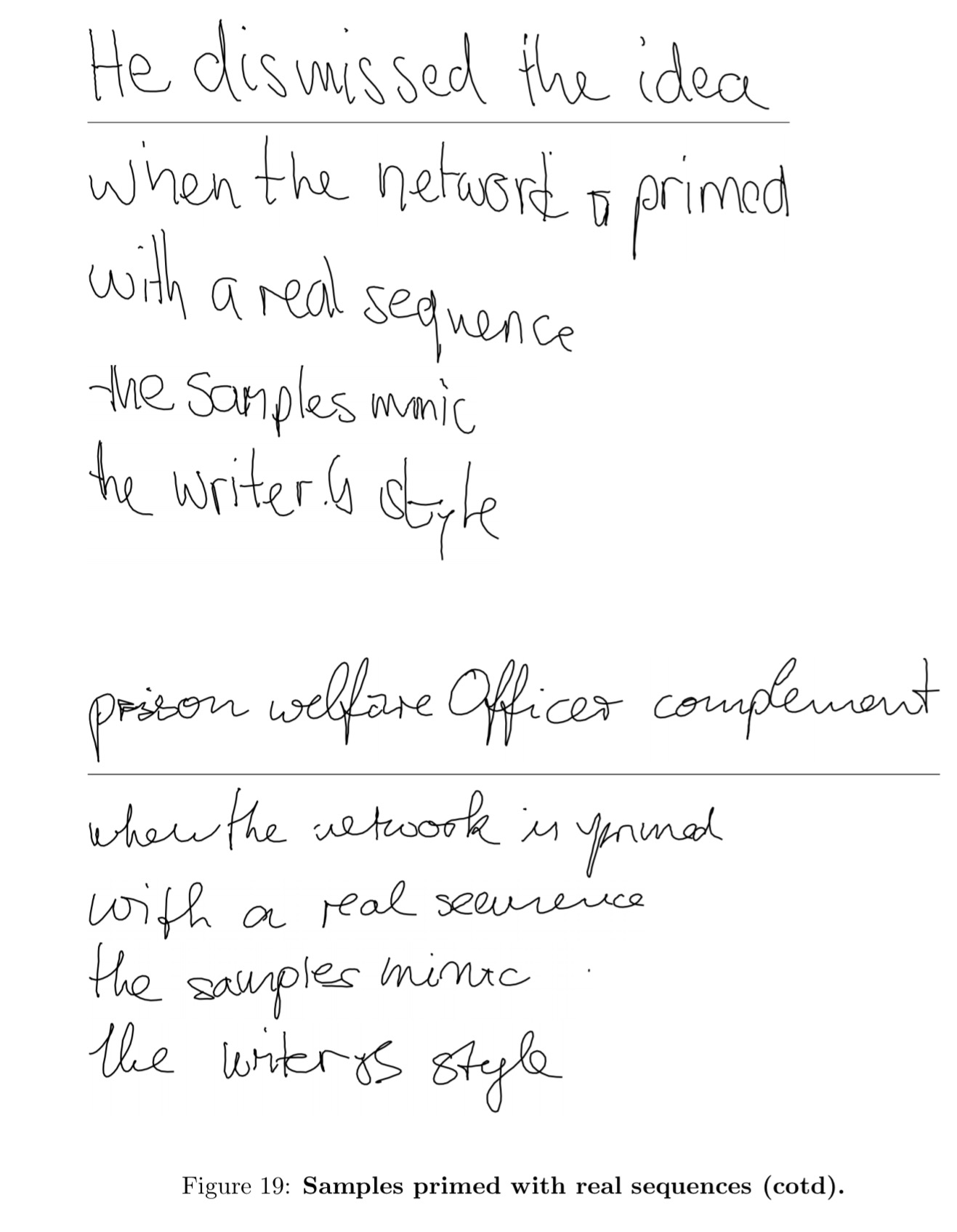
As a final flourish, we can prime the network with a real sequence in the handwriting of a particular writer. The network then continues in this style, generating handwriting mimicking the author’s style.
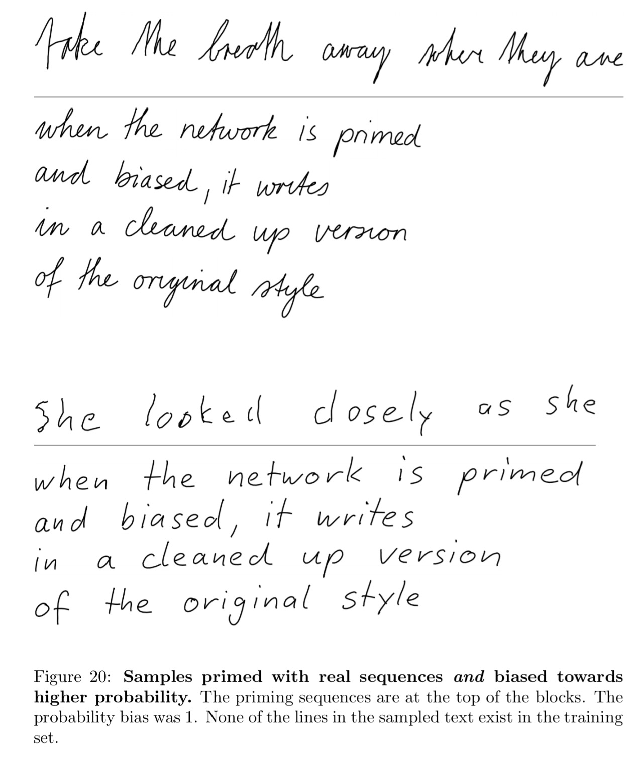
Combine this with bias, and you also get neater versions of their handwriting!
Conditional random fields as recurrent neural networks
Now we turn our attention to a new challenge problem that we haven’t looked at yet: semantic segmentation. This requires us to label the pixels in an image to indicate what kind of object they represent/are part of (land, building, sky, bicycle, chair, person, and so on…). By joining together regions with the same label, we segment the image based on the meaning of the pixels. Like this:
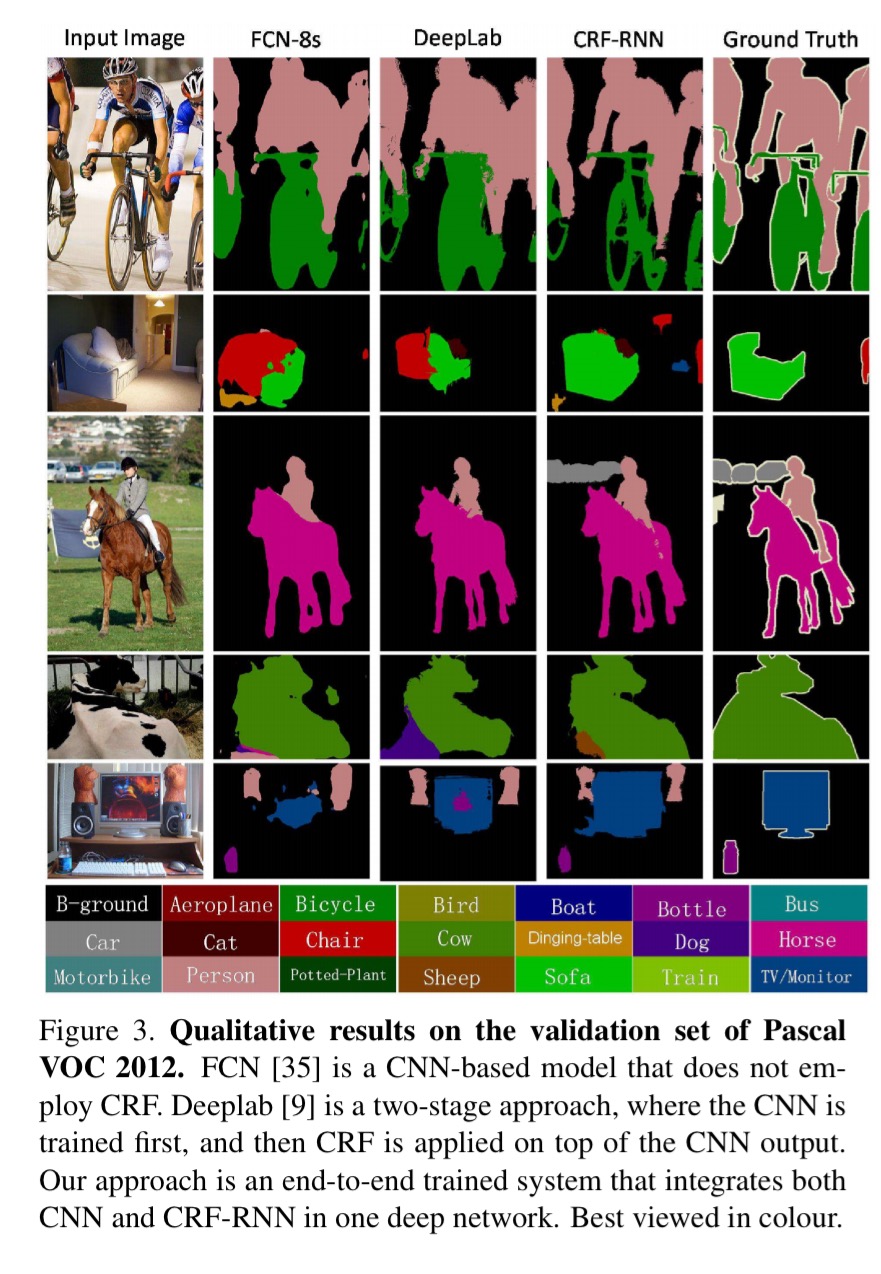
(The CRF-RNN column in the above figure shows the results from the network architecture described in this paper).
As we’ve seen, CNNs have been very successful in image classification and detection, but there are challenges applying them to pixel-labelling problems. Firstly, traditional CNNs don’t produce fine-grained enough outputs to label every pixel. But perhaps more significantly, even if we could overcome that hurdle, they don’t have any way of understanding that if pixel A is part of, say, a bicycle, then it’s likely that the adjacent pixel B is also part of a bicycle. Or in more fancy words:
CNNs lack smoothness constraints that encourage label agreement between similar pixels, and spatial and appearance consistency of the labelling output. Lack of such smoothness constraints can result in poor object delineation and small spurious regions in the segmentation output.
Conditional Random Fields (a variant of Markov Random Fields) are very good at smoothing. They’re basically models that take into account surrounding context when making predictions. So maybe we can combine Conditional Random Fields (CRF) and CNNs in some way to get the best of both worlds?
The key idea of CRF inference for semantic labelling is to formulate the label assignment problem as a probabilistic inference problem that incorporates assumptions such as the label agreement between similar pixels. CRF inference is able to refine weak and coarse pixel-level label predictions to produce sharp boundaries and fine-grained segmentations. Therefore, intuitively, CRFs can be used to overcome the drawbacks in utilizing CNNs for pixel-level labelling tasks.
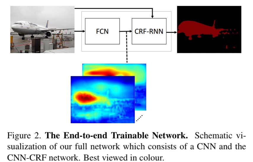
Sounds good in theory, but it’s quite tricky in practice. The authors proceed in two stages: firstly showing that one iteration of the mean-field algorithm used in CRF can be modelled as a stack of common CNN layers; and secondly by showing that repeating the CRF-CNN stack with outputs from the previous iteration fed back into the next iteration you can end up with an RNN structure, dubbed CRF-RNN, that implements the full algorithm.
Our approach comprises a fully convolutional network stage, which predicts pixel-level labels without considering structure, followed by a CRF-RNN stage, which performs CRF-based probabilistic graphical modelling for structured prediction. The complete system, therefore, unifies the strengths of both CNNs and CRFs and is trainable end-to-end using the back-propagation algorithm and the Stochastic Gradient Descent (SGD) procedure.
There’s a lot of detail in the paper, some of which passes straight over my head, for example, the following sentence which warranted me bringing out the ‘hot pink’ highlighter:
In terms of permutohedral lattice operations, this can be accomplished by only reversing the order of the separable filters in the blur stage, while building the permutohedral lattice, splatting, and slicing in the same way as in the forward pass.
(What is a permutohedron you may ask? It’s actually not as scary as it sounds…)
Fortunately, we’re just trying to grok the big picture in this write-up, and for that the key is to understand how CNNs can model one mean-field iteration, and then how we stack the resulting structures in RNN formation.
Mean-field iteration as a stack of CNN layers
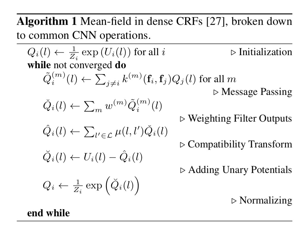
Consider a vector X with one element per pixel, representing the label assigned to that pixel drawn from some pre-defined set of labels. We construct a graph where the vertices are the elements in X, and edges between the elements hold pairwise ‘energy’ values. Minimising the overall energy of the configuration yields the most probable label assignments. Energy has two components: a unary component which depends only on the individual pixel and roughly speaking, predicts labels for pixels without considering smoothness and consistency; and pairwise energies that provide an image data-dependent smoothing term that encourages assigning similar labels to pixels with similar properties. The energy calculations are based on feature vectors derived from image features. Mean-field iteration is used to find an approximate solution for the minimal energy configuration.
The steps involved in a single iteration are:
- message passing,
- re-weighting,
- compatibility transformation,
- unary addition, and
- normalisation
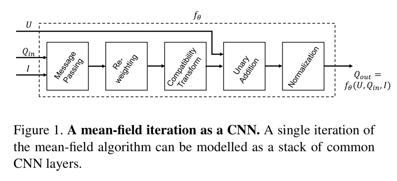
Message passing is made tractable by using approximation techniques (those permutohedral lattice thingies) and two Guassian kernels: a spatial kernel and a bilateral kernel. Re-weighting can be implemented as a 1×1 convolution. Each kernel is given independent weights:
The intuition is that the relative importance of the spatial kernel vs the bilateral kernel depends on the visual class. For example, bilateral kernels may have on the one hand a high importance in bicycle detection, because similarity of colours is determinant; on the other hand they may have low importance for TV detection, given that whatever is inside the TV screen may have different colours.
Compatibility transformation assigns penalties when different labels are assigned to pixels with similar properties. It is implemented with a convolutional filter with learned weights (equivalent to learning a label compatibility function).
The addition (copying) and normalisation (softmax) operations are easy.
CRF as a stack of CRF-CNN layers
Multiple mean-field iterations can be implemented by repeating the above stack of layers in such a way that each iteration takes Q value estimates from the previous iteration and the unary values in their original form. This is equivalent to treating the iterative mean-field inference as a Recurrent Neural Network (RNN)… We name this RNN structure CRF-RNN.
Recall that the overall network has a fully-convolution network stage predicting pixels labels in isolation, followed by a CRF-CNN for structured prediction. In one forward pass the computation goes through the initial CNN stage, and then it takes T iterations for data to leave the loop created by the RNN. One the data leaves this loop, a softmax loss layer directly follows and terminates the network.
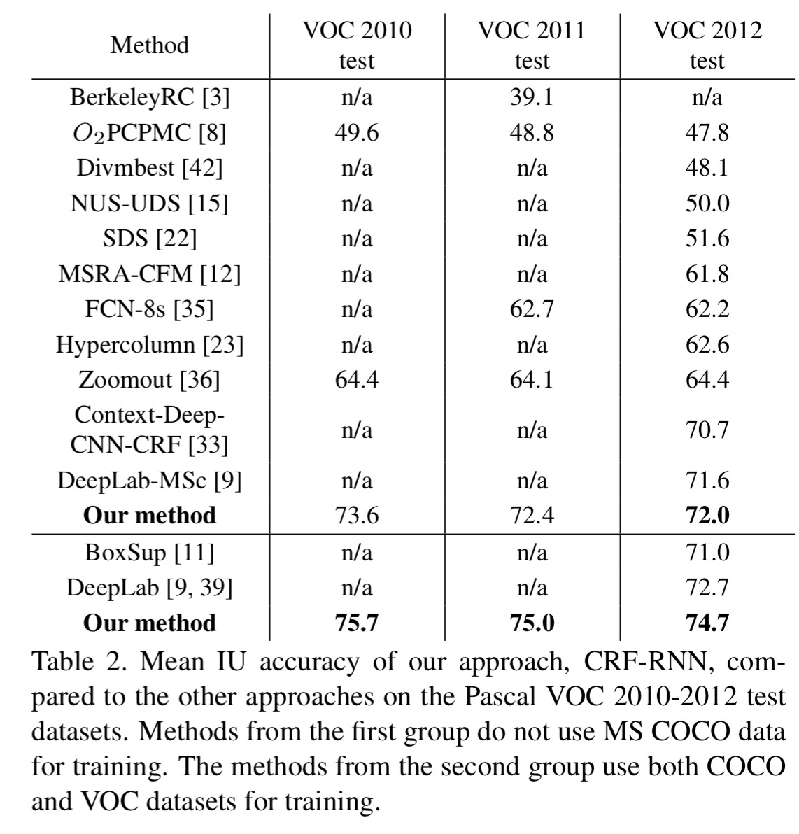
The resulting network achieves the state-of-the-art on the Pascal VOC 2010-2012 test datasets.
Nice Info