Today we’re looking at the final four papers from the ‘convolutional neural networks’ section of the ‘top 100 awesome deep learning papers‘ list.

• Deep residual learning for image recognition, He et al., 2016
• Identity mappings in deep residual networks, He et al., 2016
• Inception-v4, inception-resnet and the impact of residual connections or learning, Szegedy et al., 2016
• Rethinking the inception architecture for computer vision, Szegedy et al., 2016

Deep residual learning for image recognition

Another paper, another set of state-of-the-art results, this time with 1st place on the ILSVRC 2015 classification tasks (beating GoogLeNet from the year before), as well as 1st place on ImageNet detection, ImageNet localisation, COCO detection, and COCO segmentation competitions. For those of you old enough to remember it, there’s a bit of a Crocodile Dundee moment in this paper: “22 layers? That’s not a deep network, this is a deep network…” How deep? About 100 layers seems to work well, though the authors tested networks up to 1202 layers deep!! Which begs the question, how on earth do you effectively train a network that is hundreds or even a thousand layers deep?

Driven by the significance of depth, a question arises: Is learning better networks as easy as stacking more layers?

No, it’s not. A degradation problem occurs as network depth increases, accuracy gets saturated, and then degrades rapidly as further layers are added. So after a point, the more layers you add, the worse the error rates. For example:

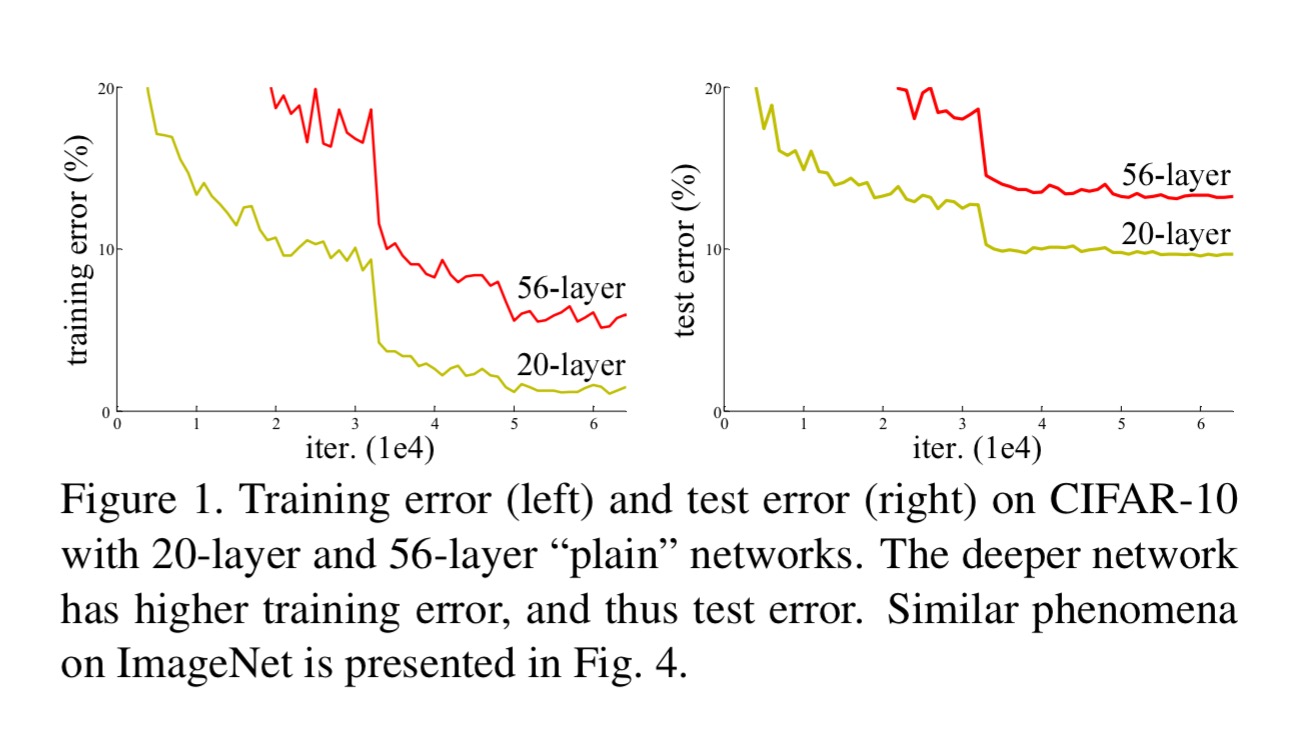
An interesting thought experiment leads the team to make a breakthrough and defeat the degradation problem. Imagine a deep network where after a certain (relatively shallow) number of layers, each additional layer is simply an identity mapping from the previous one: “the existence of this constructed solution indicates that a deeper model should produce no higher training error than its shallower counterpart.”

Suppose the desired mapping through a number of layers for certain features really is close to the identity mapping. The degradation problem suggests that the network finds it hard to learn such mappings across multiple non-linear layers. Lets say the output of one layer is . Now skip forward three layers in the network and imagine that we’d like the ability to easily learn an identity mapping (or close to) for some elements of – an easy way to do this is just to provide the elements of as direct inputs…

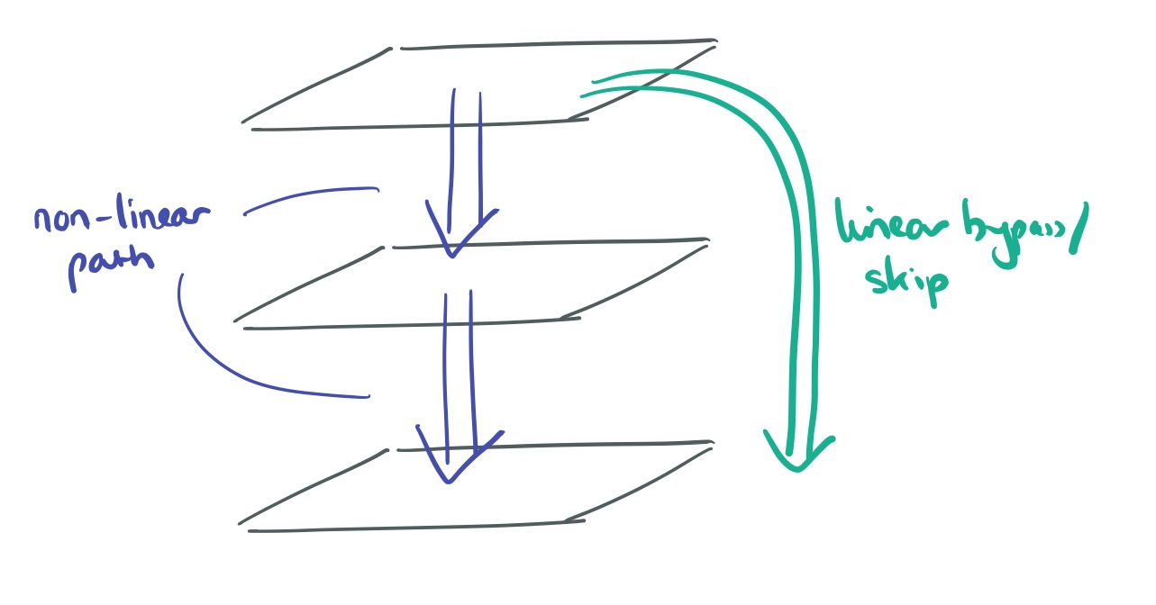
But we don’t want to just double the width of the receiving layer, and for some other elements of perhaps we do want to learn some non-linear function. So here comes the clever part: suppose the ideal function we could learn is . If the intervening hidden layers can learn that then they can also learn . Maybe you can see where this is going: we can now simply combine the output of the previous layer with using simple addition and we get ! But constructing things in this way though, we make it easy for the network to include both non-linear elements and also near identity elements (by learning weights close to zero).

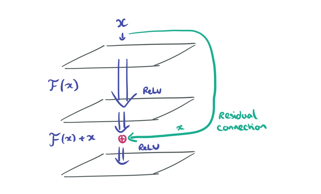
Adding these layer jumping + addition short-circuits to a deep network creates a residual network. Here’s a 34-layer example:

Here are 18 and 34 layer networks trained on ImageNet without any residual layers. You can see the degradation effect with the 34 layer network showing higher error rates.

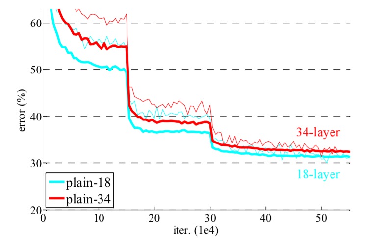
Take the same networks and pop in the residual layers, and now the 34-layer network is handsomely beating the 18-layer one.

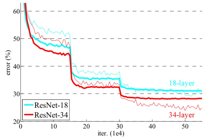
Here are the results all the way up to 152 layer networks:

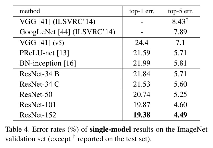
Now that’s deep!

Identity mappings in deep residual networks

This paper analyses the skip-layers introduced in the residual networks (ResNets) that we just looked at to see whether the identity function is the best option for skipping. It turns out that it is, and that using an identity function for activation as well makes residual units even more effective.

Recall that we used as the input when skipping layers. More generally, this is where h is the identity function. But h could be also be another kind of function – for example constant scaling. The authors try a variety of different h functions, but identity works best. When we consider the activation function f as well (the original paper used ReLU) then we have . Things work even better when f is also an identity mapping (instead of ReLU).

To construct an identity mapping f, we view the activation functions (ReLU and Batch Normalization) as “pre-activation” of the weight layers, in contrast to conventional wisdom of “post-activation”. This point of view leads to a new residual unit design, shown in Fig 1(b).

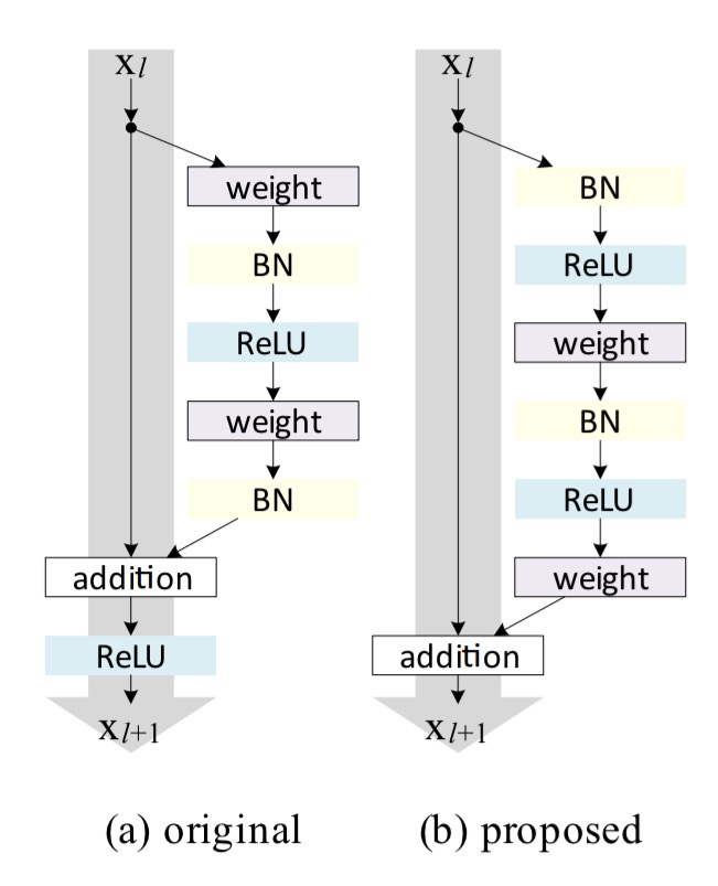
Making both h and f identity mappings allows a signal to be directly propagated from one unit to any other units, in both forward and backward passes.

Here’s the difference the new residual unit design makes when training a 1001 layer ResNet:

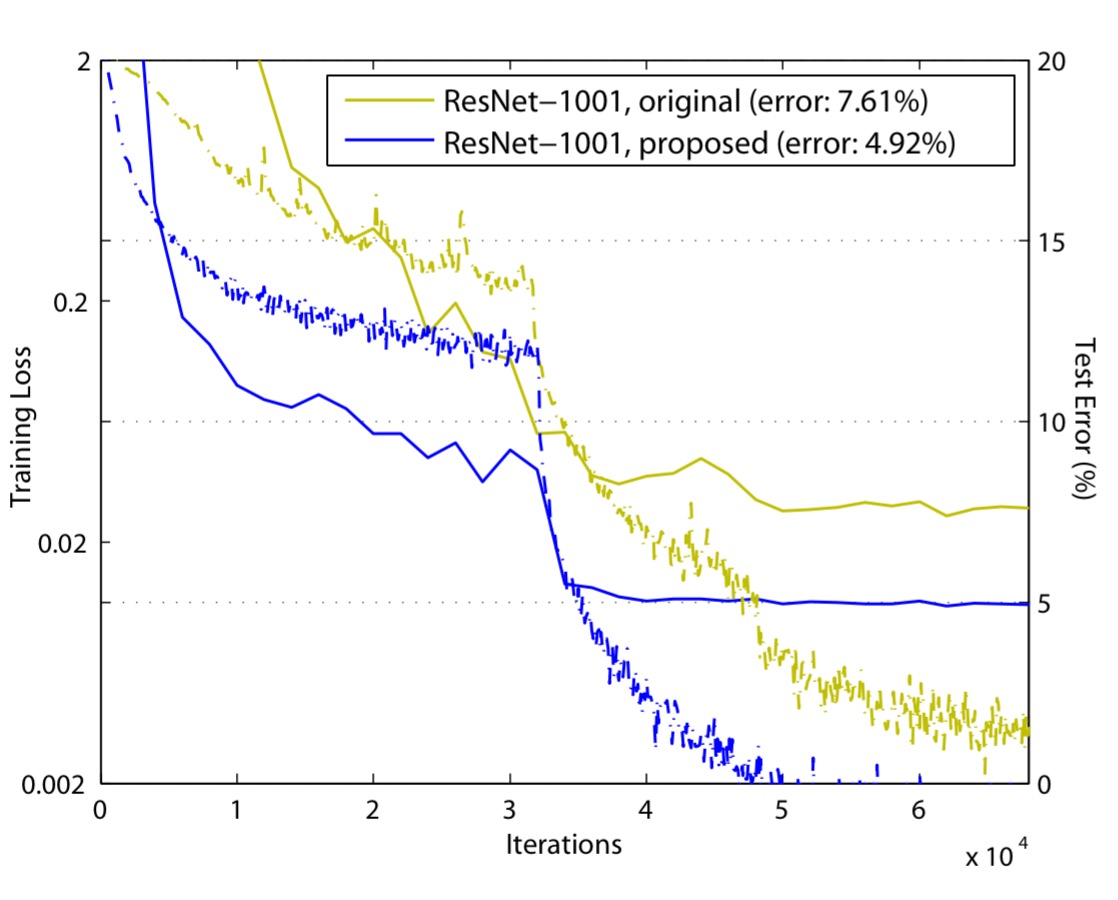
Based on this unit, we present competitive results on CIFAR-10/100 with a 1001-layer ResNet, which is much easier to train and generalizes better than the original ResNet. We further report improved results on ImageNet using a 200-layer ResNet, for which the counterpart of [the original ResNet] starts to overfit. These results suggest that there is much room to exploit the dimension of network depth, a key to the success of modern deep learning.

Inception-v4, inception-resnet and the impact of residual connections or learning

While all this ResNet excitement was going on, the Inception team kept refining their architecture, up to Inception v3. The obvious question became: what happens if we take the Inception architecture and we add residual connections to it? Does that further improve training time or accuracy? This paper compares four models: Inception v3, a newly introduced in this paper Inception v4, and variations of Inception v3 and v4 that also have residual connections. It’s also fun to see ever more complex network building blocks being used as modules in higher level architectures. Inception v4 is too much to show in one diagram, but here’s the overall schematic:

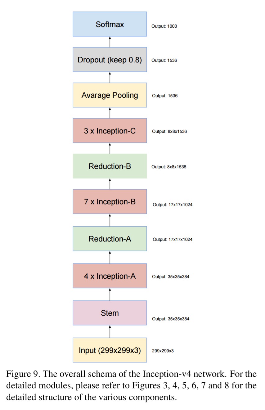
And as a representative selection, here’s what you’ll find if you dig into the stem module:

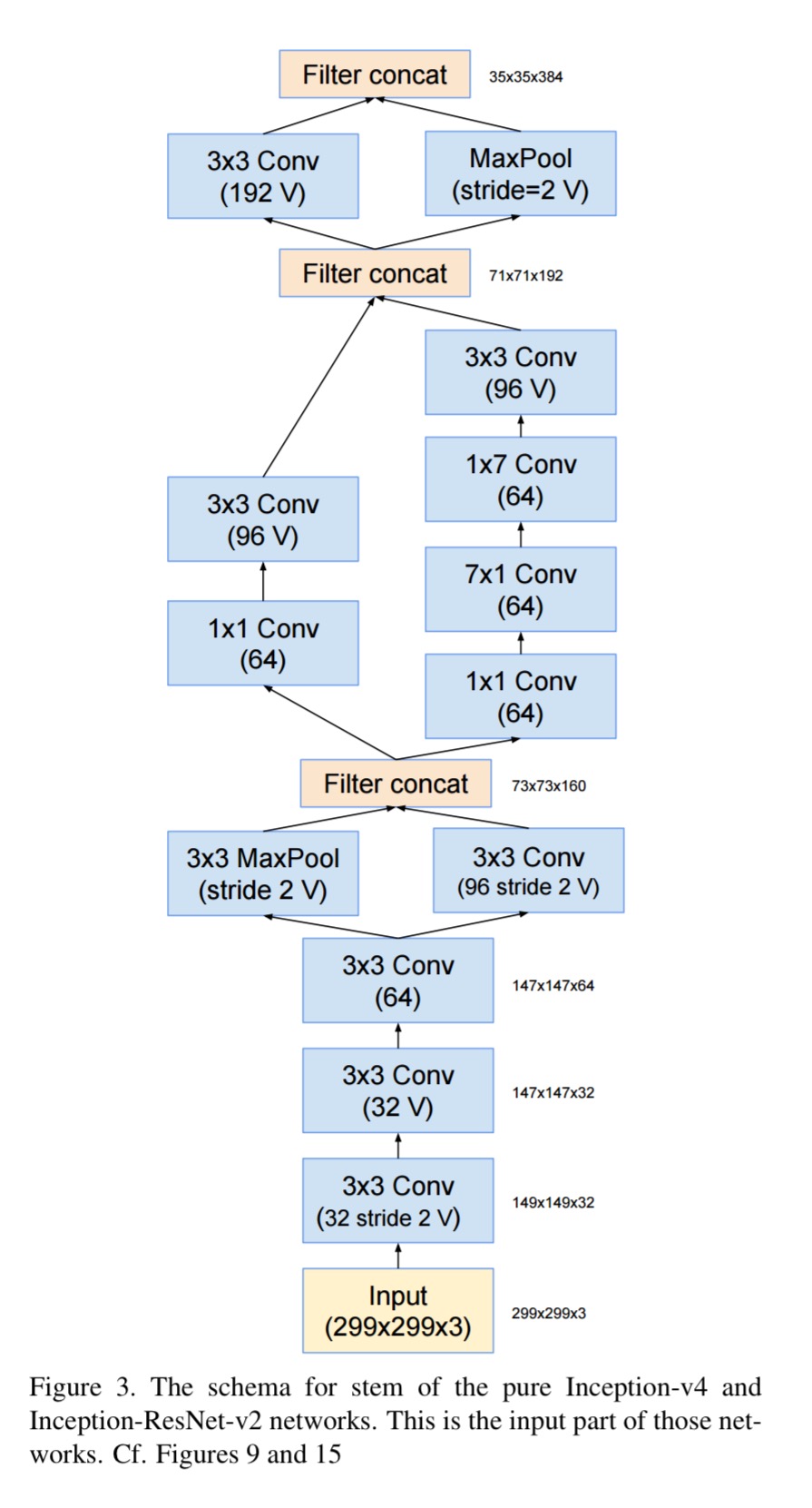
And the ’17 x 17 Inception-B’ module:

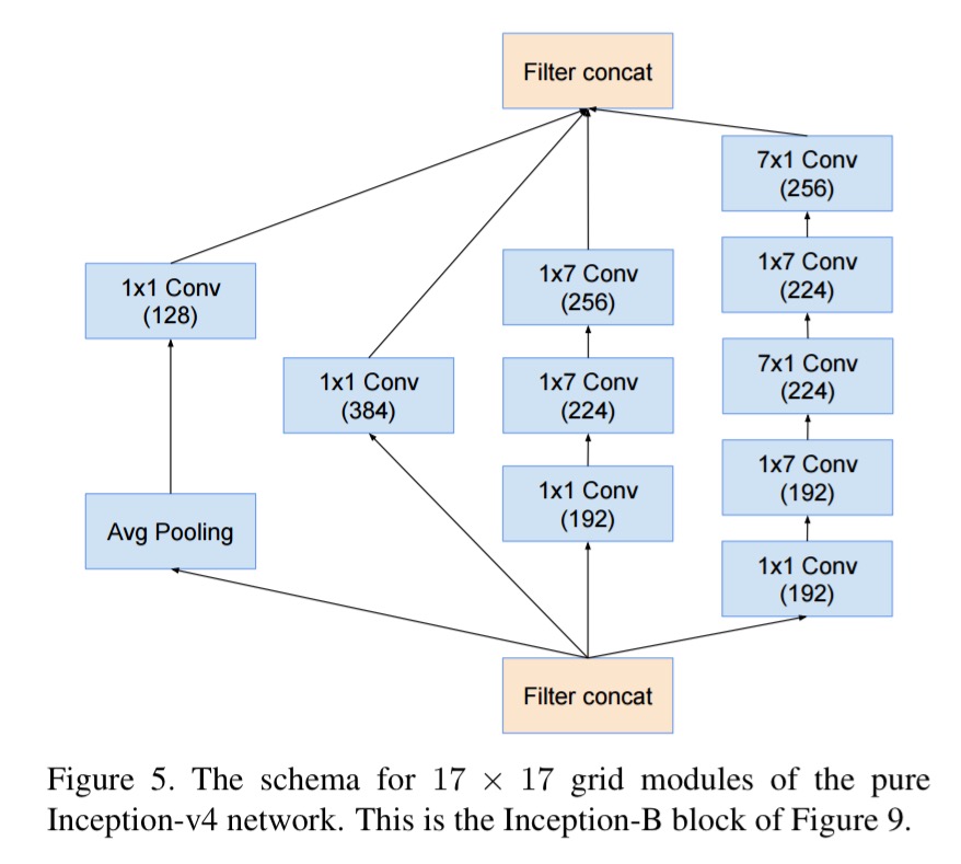
Recently, the introduction of residual connections in conjunction with a more traditional architecture has yielded state-of-the-art performance in the 2015 ILSVRC challenge; its performance was similar to the latest generation Inception-v3 network. This raises the question of whether there are any benefit in combining the Inception architecture with residual connections. Here we give clear empirical evidence that training with residual connections accelerates the training of Inception networks significantly. There is also some evidence of residual Inception networks outperforming similarly expensive Inception networks without residual connections by a thin margin.

Since Inception 4 and Inception-ResNet-v2 (Inception 4 with residual connections) give overall very similar results, this seems to suggest that – at least at this depth – residual networks are not necessary for training deep networks.

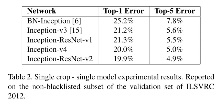
However, the use of residual connections seems to improve the training speed greatly, which is alone a great argument for their use.

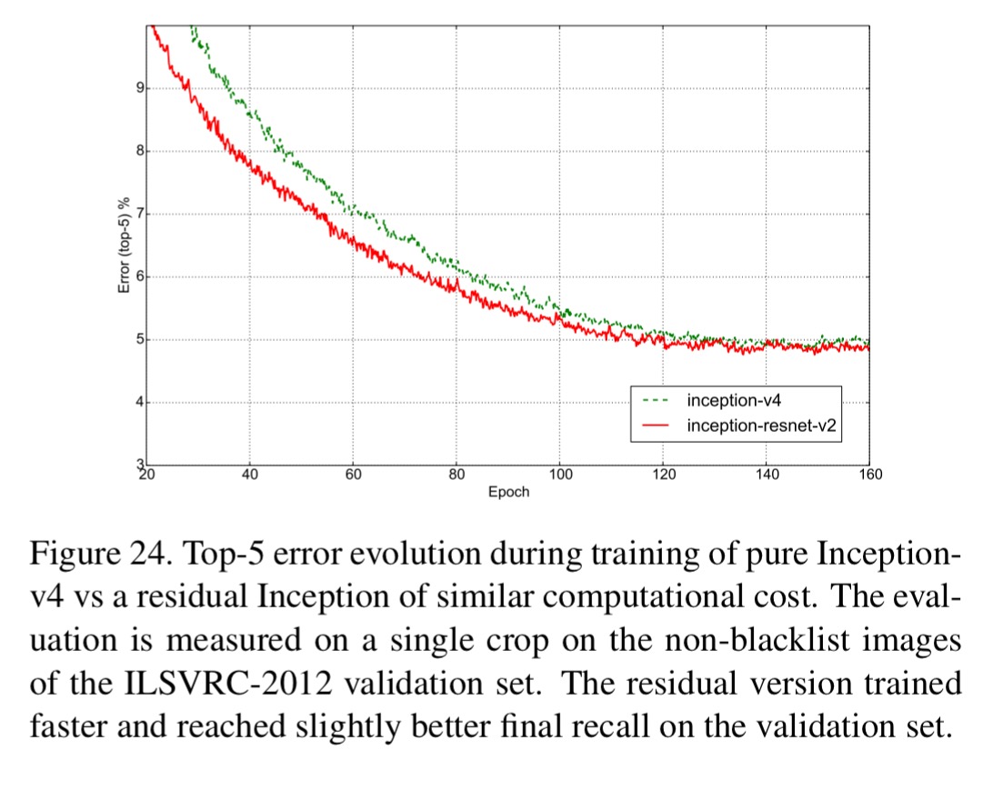
Both the Inception v4 and Inception ResNet-2 models outperform previous Inception networks, by virtue of the increased model size.

Rethinking the Inception architecture for computer vision

This paper comes a little out of order in our series, as it covers the Inception v3 architecture. The bulk of the paper though is a collection of advice for designing image processing deep convolutional networks. Inception v3 just happens to be the result of applying that advice.

In this paper, we start with describing a few general principles and optimization ideas that proved to be useful for scaling up convolution networks in efficient ways.

• Avoid representational bottlenecks – representation size should gently decrease from the inputs to the outputs before reaching the final representation used for task at hand. Big jumps (downward) in representation size cause extreme compression of the representation and bottleneck the model.
• Higher dimensional representationsare easier to process locally in a network, more activations per tile allows for more disentangled features. The resulting networks train faster.
• Spatial aggregation of lower dimensional embeddings can be done without much or any loss in representational power. “For example, before performing a more spread out (e.g. 3×3 convolution), one can reduce the dimension of the input representation before the spatial aggregation without expecting serious adverse effects.”
• Balance network width and depth, optimal performance is achieved by balancing the number of filters per stage and the depth of the network. I.e., if you want to go deeper you should also consider going wider.

Although these principles might make sense, it is not straightforward to use them to improve the quality of networks out of the box. The idea is to use them judiciously in ambiguous situations only.

• Factorize into smaller convolutions, a larger (e.g. 5×5) convolution is disproportionately more expensive than a smaller (e.g. 3×3) one – by a factor of 25/9 in this case. Replacing the 5×5 convolution with a two-layer network of 3×3 convolutions reusing activations between adjacent tiles achieves the same end but uses (9+9)/25 less computation.

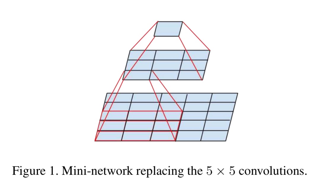
The above results suggest that convolutions with filters larger 3 × 3 a might not be generally useful as they can always be reduced into a sequence of 3 × 3 convolutional layers. Still we can ask the question whether one should factorize them into smaller, for example 2×2 convolutions. However, it turns out that one can do even better than 2 × 2 by using asymmetric convolutions, e.g. n × 1. For example using a 3 × 1 convolution followed by a 1 × 3 convolution is equivalent to sliding a two layer network with the same receptive field as in a 3×3 convolution. The two-layer solution is 33% cheaper.

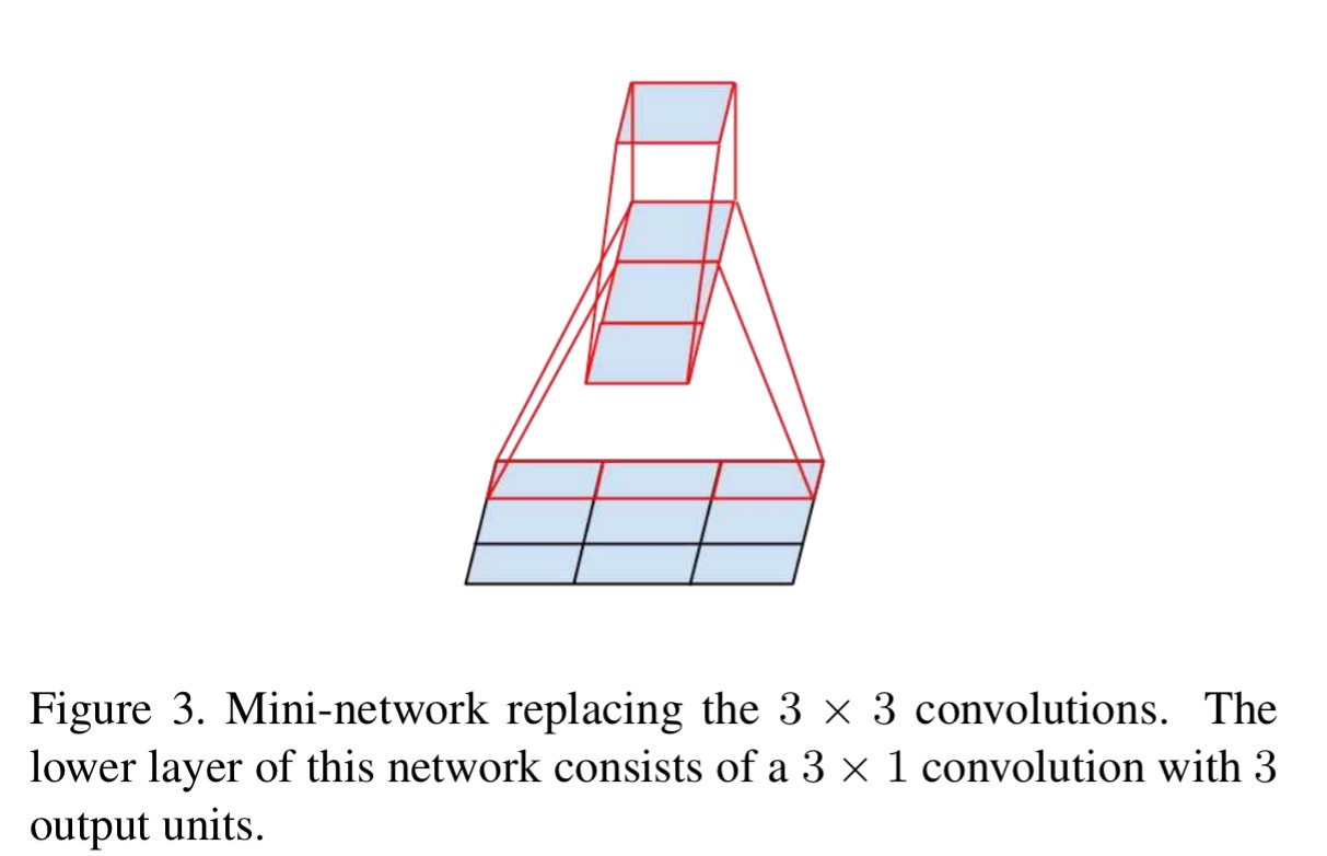
Taking this idea even further (e.g. replacing 7×7 with a 1×7 followed by a 7×1) works well on medium grid sizes (between 12 and 20), so long as it is not used in early layers.

The authors also revisit the question of the auxiliary classifiers used to aid training in the original Inception. “Interestingly, we found that auxiliary classifiers did not result in improved convergence early in the training… near the end of training the network with the auxiliary branches starts to overtake the accuracy of the network without, and reaches a slightly higher plateau.” Removing the lower of the two auxiliary classifiers also had no effect.

Together with the earlier observation in the previous paragraph, this means that original the hypothesis of [Inception] that these branches help evolving the low-level features is most likely misplaced. Instead, we argue that the auxiliary classifiers act as regularizer.

There are several other hints and tips in the paper that we don’t have space to cover. It’s well worth checking out if you’re building these kinds of models yourself.