Time series classification under more realistic assumptions – Hu et al. ICDM 2013
This paper sheds light on the gap between research results in time series classification, and what you’re likely to see if you try to apply the results in the real world. And having identified the gap of course, the authors go on to greatly reduce it…
In virtually all time series classification research, long time series are processed into short equal-length “template” sequences that are representative of the class… [and researchers work with] perfectly aligned data, containing all of the target behavior and only the target behavior. Unsurprisingly, dozens of papers report less than 10% classification eror rate on this problem. However, does such an error rate reflect our abilities with real-world data? … We believe that such contriving of the data has led to unwarranted optimism about how well we can classify real-time series data streams. For real-world problems, we cannot always expect the training data to be so idealized, and we certainly cannot expect the testing data to be so perfect.
Three assumptions (or at least one of these three assumptions) underpin much of the progress in time series classification in the decade preceding this paper:
- Copious amounts of perfectly aligned atomic patterns can be obtained
- The patterns are all of equal length
- Every item we attempt to classify belongs to exactly one of our well defined classes
To simplify things for a moment consider a toy example in a small discrete domain (the real goal is large real-valued time series data). We have gait data, and we want to classify it as ‘walk’, ‘run’, or ‘sprint’. The patterns are going to need to be the same length, so let’s actually look for ‘walk’, ‘rrun’, and ‘sprt.’ Every item would need to belong to exactly one of these classes, so fast walking is probably ok, but jogging would be right out. And finally we assume copious amounts of perfectly aligned atomic patterns, so we want training data that looks something like this:
Class 1: 'walkwalkwalkwalkwalk...'
Class 2: 'rrunrrunrrunrrunrrun...'
Class 3: 'sprtsprtsprtsprt...'
In the real-world, we tend to have weakly-labelled time series annotated by behaviour or some other mapping to the ground truth. “By weakly-labelled, we simply mean that each long data sequence has a single global label and not lots of local labelled pointers to every beginning and ending of individual patterns, e.g. individual gestures.” Such data has two important properties:
- It will contain extraneous / irrelevant sections – for example during a gait recording session a subject may pause to cross a road, or jump over a puddle. Such phenomena appear in all the datasets examined by the authors.
- It will contain lots of significant redundancies: “while we want lots of data in order to learn the inherent variability of the concept we wish to learn, significant redundancy will make our classification algorithms slow once deployed.”
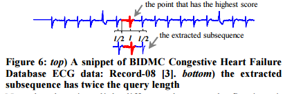
The following ECG trace exhibits both of these properties:
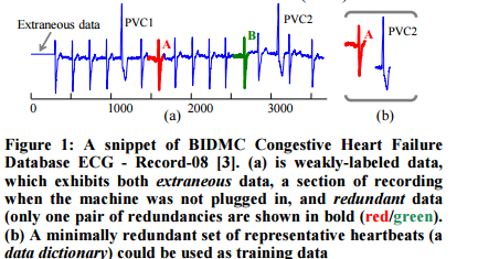
The authors develop a technique by which a real world time series can be preprocessed to eliminate extraneous sections and redundancy – without requiring human intervention to edit the time series by hand. The ideal training set would contain no spurious data, and exactly one instance of each of the ways the target behaviour is manifest. This idealised training set is called a data dictionary.
Given a data dictionary, a classifier can determine the class membership of a query using a straightforward nearest neighbour approach and a threshold:
- If the query’s nearest neighbour distance is larger than the threshold distance, then we say that the query does not belong to any class in the data dictionary, otherwise…
- The query is assigned to the same class as its nearest neighbour.
Best results are achieved using a Uniform Scaling distance rather than a Euclidean distance.
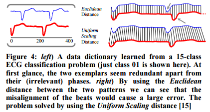
We have found that using the Uniform Scaling distance allows us to have a significantly smaller data dictionary… beyond reducing the size of data dictionaries (thus speeding up classification), there is an additional advantage of using Uniform Scaling; it allows us to achieve a lower error rate. How is this possible? It is possible because we can generalize to patterns not seen in the training data.
Classification using data dictionaries produces much lower error rates than the previous state of the art, while also being much faster since only a small fraction of the overall data needs to be examined. For example, in a physical activity data set traditional approaches use all of the training data and achieve a testing error rate of 0.221. The data dictionary approach can achieve the same error rate by examining only 1.6% of the training data! And it can achieve the much lower 0.085 error by looking at only 8.1% of the training data. In a cardiology dataset test, the authors achieved a 0.035 testing error rate using only 4.6% of the training data set (vs the default error rate of 0.933 with prior approaches, when using all of the training data).
The classification errors are reduced because the data dictionary contains less spurious, and therefore potentially misleading, data. And the redundancy in most time series means that in most real-world problems the data dictionary can be aronud 5% of the size of the full training data, and still be at least as accurate as approaches that use all of it.
With less than one tenth of the original data kept in [the data dictionary], we are at least ten times faster at classification time.
Better, faster, cheaper classification that works with real-world data sets sounds pretty attractive. So let’s take a look at how to build a data dictionary…
Creating an ideal training set from weakly-labeled time series
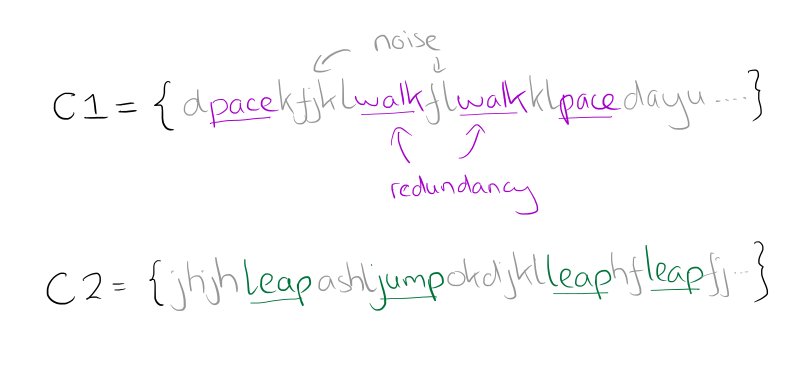
Let’s continue with the easier to understand discrete domain example. In the paper, the authors describe a training dataset in which we wish to distinguish between two classes, C1 and C2. We have weakly labeled data for each class:
C1 = {dpacekfjklwalkflwalkklpacedalyutexwalksfj }
C2 = { jhjhleapashljumpokdjilleaphfleapfjumpacgd }
The true subsequences that we really want to learn are that ‘pace’ and ‘walk’ indicate a subsequence belonging to C1, and ‘leap’ and ‘jump’ indicate a subsequence belong to C2. It can be clearly seen that the training data contains both extraneous and redundant data:
The data dictionary D should be the following:
D = C1 : { pace; walk } C2 : { leap ; jump }, r = 1
r is the rejection threshold distance – in this case we consider a subsequence to be a class match if it is within (hamming) distance of 1. So an incoming query of ieap would be matched as class C2, but a query of kklp would be rejected. The second example is especially interesting, because it actually appears in C1 ‘by accident’ which could have led to a misclassification if using the full training dataset.
This misclassification is clearly contrived, but it does happen frequently in the real data… In our example we have considered two separate queries; however a closer analogue of our real-valued problem is to imagine an endless stream that needs to be classified: …ttgpacedgrteweerjumpwalkflqrafertwqhafhfahfahfbseew…
The creation of the data dictionary is based on ranking and scoring candidate substrings using leaving-one-out classification.
For example, by using leaving-one-out to classify the first substring of length 4 in C1 dpac, it is incorrectly classified as C2 (it maches the middle of ..umpacgd.. with a distance of 1). In contrast, when we attempt to classify the second substring of length 4 in C1, pace, we find it is correctly classified. By collecting statistics about which substrings are often used for correct predictions, but rarely used for wrong predictions, we find that the four substrings shown in our data dictionary emerge as the obvious choices. This basic idea is known as data editing.
The algorithm proceeds iteratively, in each iteration:
- Score the subsequences in C. Scoring is based on a combination of classification error rate, and how close (nearest neighbour distance) the sequence is to ‘friend’ objects with the same class label vs ‘enemy’ objects with different class labels.
- Extract the highest scoring subsequence and place it in D
- Identify all queries that cannot be correctly classified by the current D, use these to rescore the subsequences in C in the next iteration.
Step 3 is key to reducing redundancy in D. Suppose one of the walk subsequences in C1 has scored the highest in the current iteration and been placed into D. By removing all of the queries that can be correctly classified by this subsequence, it means that the other walk subsequences in C1 will score lower in subsequent iterations.
The process iterates until we run out of subsequences to add to D or the unlikely event of perfect training error rate having been achieved. In the dozens of problems we have considered, the training error rate plateaus well before 10% of the training data has been added to the data dictionary.
To reduce sensitivity to misalignments the chosen subsequence (in step 2) is padded with extra points from the left and the right. For query length l, l/2 data points are used on each side.
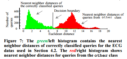
Once the data dictionary is built, the threshold used to reject future queries which do not belong to any of the learned classes is determined. Two histograms are computed, one for the nearest neighbour distances of queries that are correctly classified using D, and one for the nearest neighbour distances of queries that should not have a valid match within D (you can get such queries from some other unrelated dataset for example).
Given the two histograms, we choose the location that gives the equal-error-rate as the threshold. However, based on their tolerance to false negatives, users may choose a more liberal or conservative decision boundary.