The Data Calculator: data structure design and cost synthesis from first principles and learned cost models Idreos et al., SIGMOD’18
This paper preceded the work on data continuums that we looked at last time, and takes a more general look at interactive and semi-automated design of data structures. A data structure here is defined as a combination of (1) a data layout describing how the data is stored, and (2) algorithms that describe how its basic functionality is achieved over the specific data layout. For data structures with just two different types of nodes (e.g., leaf-nodes and non-leaf nodes in a tree), the authors estimate there are more than possible valid data structure designs! Dozens of new data structures are published each year, but we’re still only scratching the surface.
Our intuition as that most designs (and even inventions) are about combining a small set of fundamental concepts in different ways or tunings… Our vision is to build the periodic table of data structures so we can express their massive design space. We take the first step in the paper, presenting a set of first principles that can synthesize an order of magnitude more data structure designs than what has been published in the literature.
Alongside the ability to synthesise data structure designs the authors also build a cost model so that designs can be evaluated and ranked. The cost model is informed by a combination of analytical models, benchmarks, and machine learning for a small set of fundamental access primitives.
The design primitives and cost model are brought together in a tool called the ‘Data Calculator’, which computes the performance of arbitrary data structure designs as combinations of the primitives.
It is an interactive tool that accelerates the process of design by turning it into an exploration process, improving the productivity of researchers and engineers; it is able to answer what-if data structure design questions to understand how the introduction of new design choices, workloads, and hardware affect the performance (latency) of an existing design. It currently supports read queries for basic hardware conscious layouts.

(Enlarge)
Data layout primitives
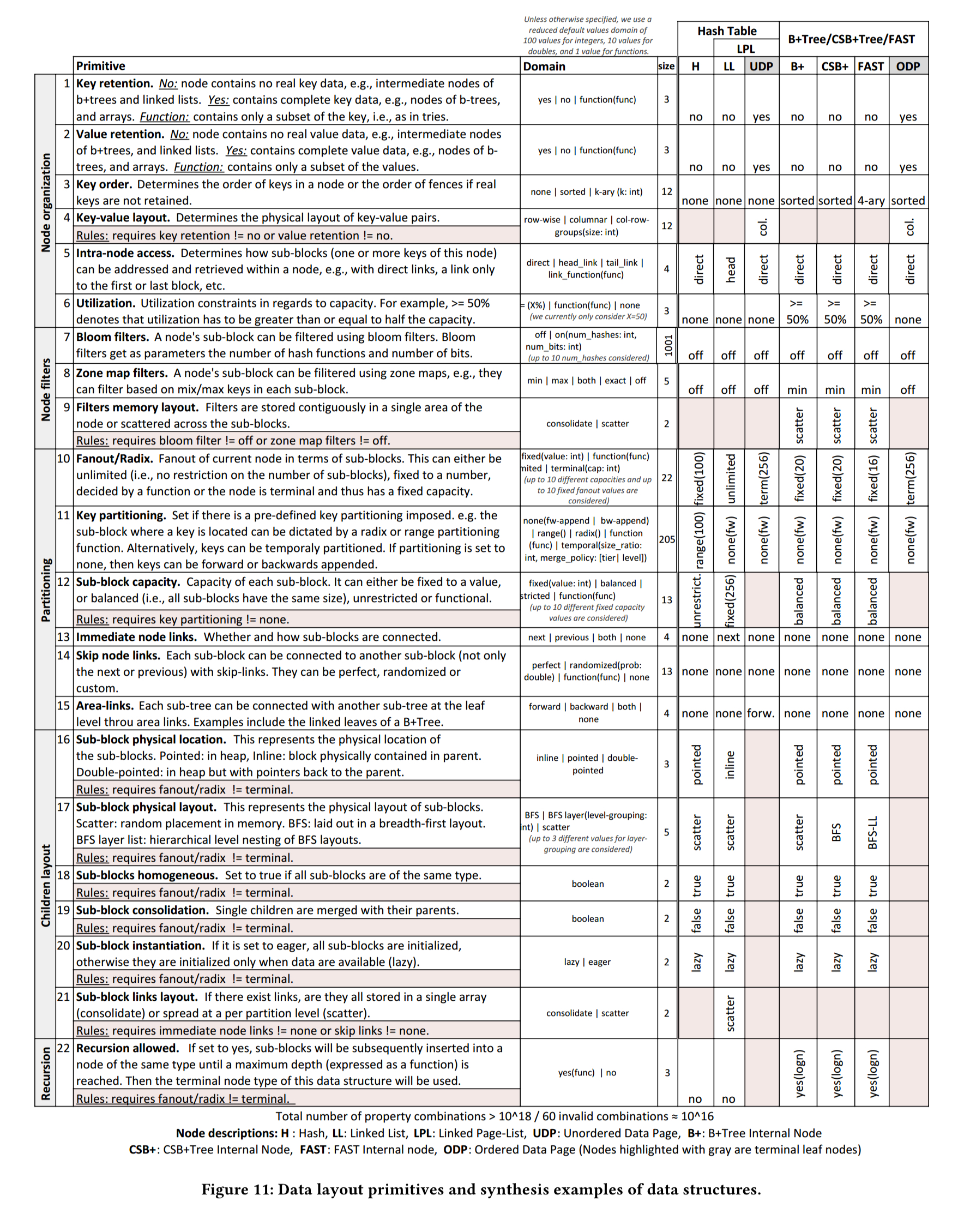
At the core of the Data Calculator are a set of design primitives, organised into five different groups (classes): how nodes are organised, filtered, and partitioned, the layout of child nodes, and whether or not recursion is allowed. Scanning the ‘domain’ column in the table below, these read like configuration parameters for a data structure generator. (The rightmost columns show the parameter values used by some common data structures – see the key at the bottom of the table). The primitives for dictating physical placement are critical to computing the cache-friendliness of a data structure, and hence the cost of traversing it.
(Enlarge)
As an example, a B+ tree uses sorted nodes with key retention none for internal nodes (they only store fences and pointers), and full for leaf nodes.
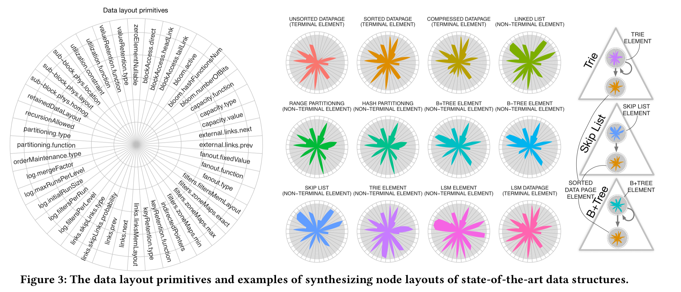
Primitives combine to form ‘elements’: the full specification of a node type within the data structure. For example, internal (non-terminal) elements and leaf (terminal) elements. Radar plots which show the design primitives selected, and the particular configuration choice made for that primitive (the segments on the radii) can be used to visually compare designs.
(Enlarge)
For two-element structures the design space describes possible designs, and for three-element structures (e.g. MassTree) there are
possibilities. The Data Calculator tool provides guidance to help navigate the design space, and test a given design against a workload and hardware setting.
How much is that data structure in the window?
Traditional cost analysis in systems and data structures happens through experiments and the development of analytical cost models. Both options are not scalable when we want to quickly test multiple different parts of the massive design space we define in this paper.
Each data access primitive characterises one aspect of how data is accessed (e.g. binary search, scan, …), and has a number of different possible embodiments (‘level 2 primitives’). The idea is to model the behaviour of these level 2 primitives, and then combine the models to understand the behaviour of data structures synthesised from combinations of the primitives.
For every level 2 primitive, the Data Calculator contains one or more models that describe its performance (latency) behavior. These are not static models; they are trained and fitted for combinations of data and hardware profiles as both these factors drastically affect performance…. The models are simple parametric models; given the design decision to keep primitives simple (so they can be easily reused), we have domain expertise to expect how their performance behavior will look like (sic).
The access primitives the types of models used for them are shown in the following table.

(Enlarge)
For example, when binary searching a sorted array we know that it should take time , and the model to be fitted is of the form
, where
,
and
are coefficients learned through linear regression.

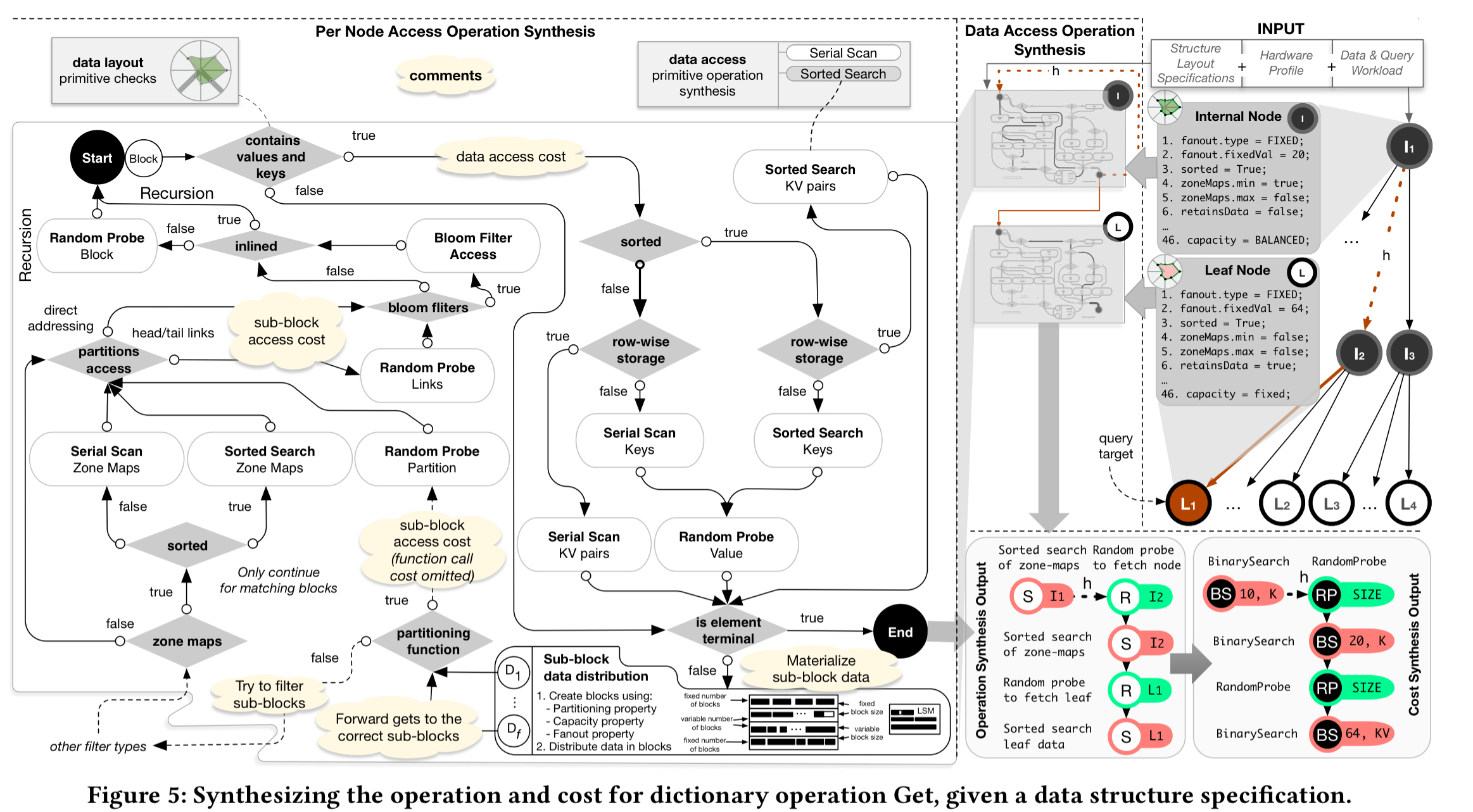
Given a data layout specification, hardware profile, and a workload, the calculator uses a rule-based system to compute the overall cost of an operation. The following figure, which should be read starting from the top-right, shows the process for estimating the cost of a Get operation. As part of the process the calculator simulates populating the data structure to figure out how many nodes will exist, the height of the structure, and so on. These information is needed to estimate the operation cost. The output is an abstract syntax tree with the access patterns of the path that needed to be traversed. These can be costed using the fitted models, and the overall cost is calculated as their sum.
(Enlarge)
A key part of figuring out performance is whether data is ‘hot’ or ‘cold’, and if it’s hot, where it sits in the cache hierarchy. The modelling intuition is that we’ll see step-like performance changes at each cache level depending on whether or not the data is cached there. We can therefore model each layer with a sigmoid function, and the overall behaviour across a cache hierarchy as the sum of a set of sigmoid functions.

For a given workload, the calculator figures out how many times each node is going to be accessed, allowing us to compute a popularity factor p: the number of accesses for the given node, divided by the total number of accesses across all nodes. The random access cost for an operation is then derived from the fitted cache model and a weighting factor . The parameter
is the cycling sequence number of the operation in the workload. The end result is that we predict smaller access costs for more frequently accessed nodes, and vice-versa.
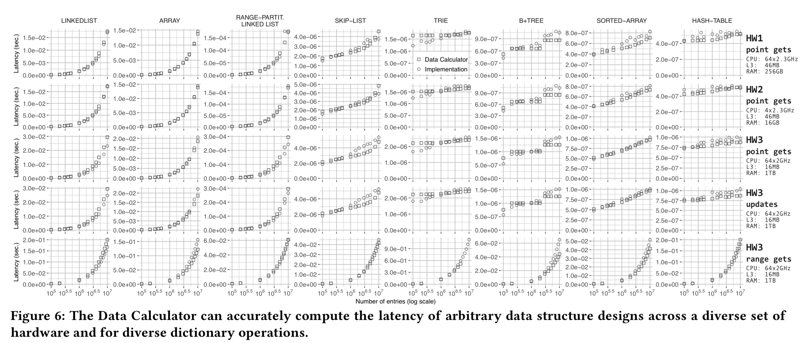
The evaluation shows that the calculator does a good job of estimating latency for a variety of different data structure designs (columns in the figure below), and hardware (the rows).
(Enlarge)
Answering ‘what-if?’ questions
By varying the input parameters to the calculator we can ask ‘what-if?’ questions. For example, “what would be the performance impact if I change my B-tree design by adding a bloom filter in each leaf?”, or “what would be the performance impact if I switched to this instance type on AWS?”. Training the level 2 primitives on a new hardware platform takes only a few minutes, and is a one-off task for each platform.
The evaluation gives an indication of the power of being able to ask these kinds of questions using a design based on a B-tree and a workload of uniform data and queries with 1 million inserts and 100 Gets:
- It takes only 20 seconds to assess the impact of a hardware change, revealing in this case that performance would drop.
- It takes 47 seconds to then ask, “if I do move to that hardware, is there a better choice of data structure?” (The search was restricted to exploring just five possible elements).
- It takes 20 seconds to confirm a hypothesis that adding a Bloom filter in all B-tree leaves would be beneficial.
- It takes 24 seconds to explore what would happen if skew is introduced into the workload (performance suffers with the current design), and a further 47 seconds to compute changes that will yield better performance with the skewed workload.
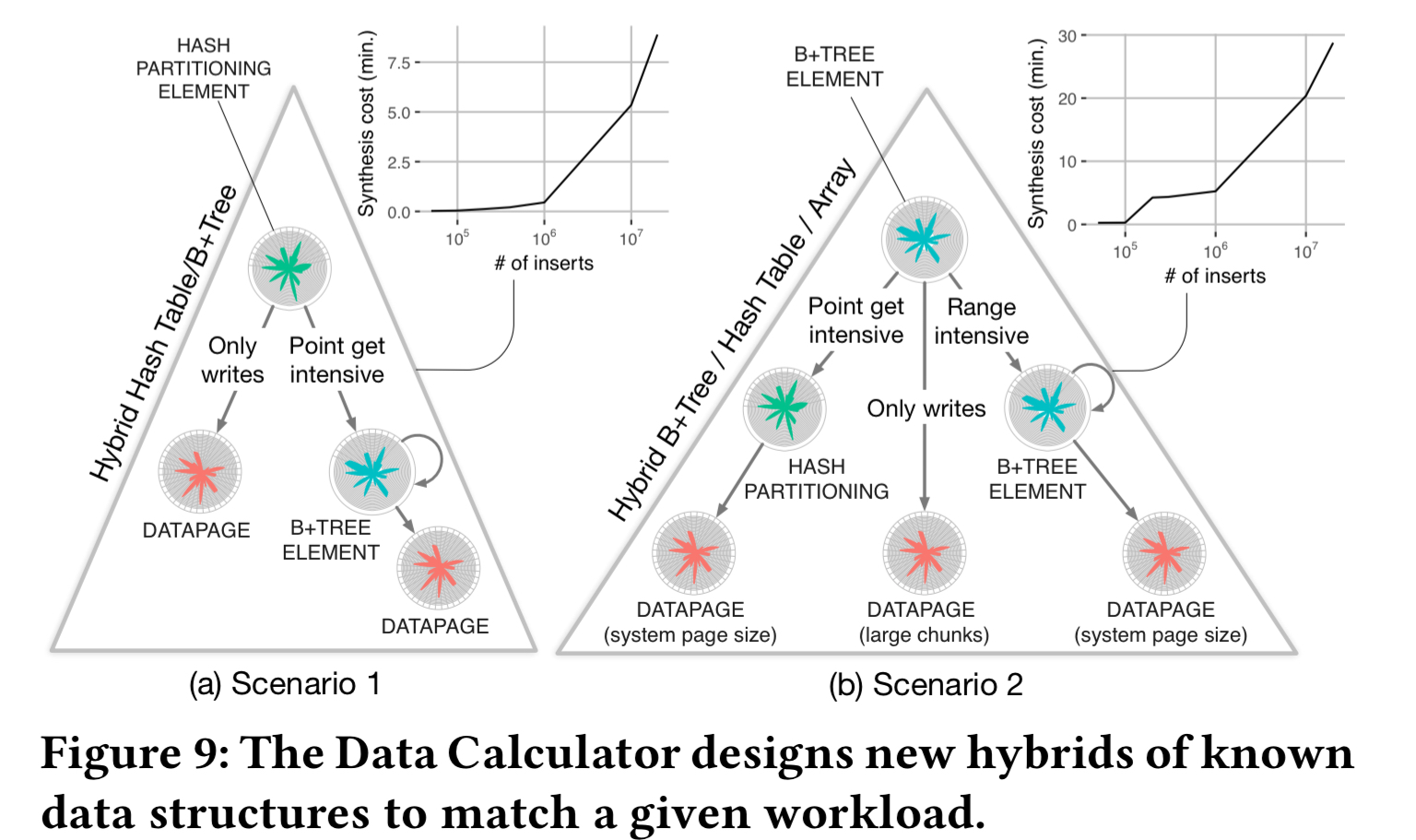
For the final part of the evaluation, the Design Calculator is asked to come up with designs for two different workload scenarios, on the same hardware profile, starting from a blank slate. The calculator is however given guidance to explore designs that combine hashing, B-Tree like indexing, and a simple log. The synthesis costs vary based on the estimated workload size: from a few seconds to 30 minutes. ”
Thus, the Data Calculator quickly answers complex questions that would normally take humans days or even weeks to test fully.
In the first scenario there are mixed reads and writes, with all reads being point queries in 20% of the domain. The calculator finds a design that use hashing at the upper levels of the hierarchy for fast access to data, but then most of the remaining domain is modelled using simple unsorted pages, with B+-tree style indexing for the read intensive part.
In the second scenario 50% of reads are point reads touching 10% of the domain, and the other 50% are range queries touching a different 10% of the domain. The calculator chooses to use hashing for the part of the domain receiving point queries, and B+-tree style indexing for the range query part.
The quest for the first principles of data structures needs to continue to find the primitives for additional significant classes of designs including updates, compression, concurrency, adaptivity, graphs, spatial data, version control management, and replication.
[confidentiality,…?]
10 thoughts on “The data calculator: data structure design and cost synthesis from first principles and learned cost models”
Comments are closed.