Filter before you parse: faster analytics on raw data with Sparser Palkar et al., VLDB’18
We’ve been parsing JSON for over 15 years. So it’s surprising and wonderful that with a fresh look at the problem the authors of this paper have been able to deliver an order-of-magnitude speed-up with Sparser in about 4Kloc.
The classic approach to JSON parsing is to use a state-machine based parsing algorithm. This is the approach used by e.g. RapidJSON. Such algorithms are sequential and can’t easily exploit the SIMD capabilities of modern CPUs. State of the art JSON parsers such as Mison are designed to match the capabilities of modern hardware. Mison uses SIMD instructions to find special characters such as brackets and colons and build a structural index over a raw json string.
… we found that Mison can parse highly nested in-memory data at over 2GMB/s per core, over 5x faster than RapidJSON, the fastest traditional state-machine based parser available.
How can we parse JSON even faster? The key lies in re-framing the question. The fastest way to parse a JSON file is not to parse it at all. Zero ms is a hard lower bound ;). In other words, if you can quickly determine that a JSON file (or Avro, or Parquet, …) can’t possible contain what you’re looking for then you can avoid parsing it in the first place. That’s similar to the way that we might use a bloom filter to rule out the presence of a certain key or value in a file (guaranteeing no false-negatives, though we might have false positives). Sparser is intended for use in situations where we are interacting directly with raw unstructured or semi-structured data though where a pre-computing index or similar data structure either isn’t available or is too expensive to compute given the anticipated access frequency.
In such a context we’re going to need a fast online test with no false negatives. Comparing state-of-the-art parsers to the raw hardware capabilities suggests there’s some headroom to work with:
Even with these new techniques, however, we still observe a large memory-compute performance gap: a single core can scan a raw bytestream of JSON data 10x faster than Mison parses it. Perhaps surprisingly, similar gaps can occur even when parsing binary formats that require byte-level processing, such as Avro and Parquet.
Imagine I have a big file containing tweet data. I want to find all tweets mentioning the hashtag ‘#themorningpaper’. Instead of feeding the file straight into a JSON parser, I could just do a simple grep first. If grep finds nothing, we don’t need to parse as there won’t be any matches. Sparser doesn’t work exactly like this, but it’s pretty close! In place of grep, it uses a collection of raw filters, designed with mechanical sympathy in mind to make them really efficient on modern hardware. A cost optimiser figures out the best performing combination of filters for a given query predicate and data set. When scanning through really big files, the cost optimiser is re-run whenever parsing throughput drops by some threshold (20% in the implementation).
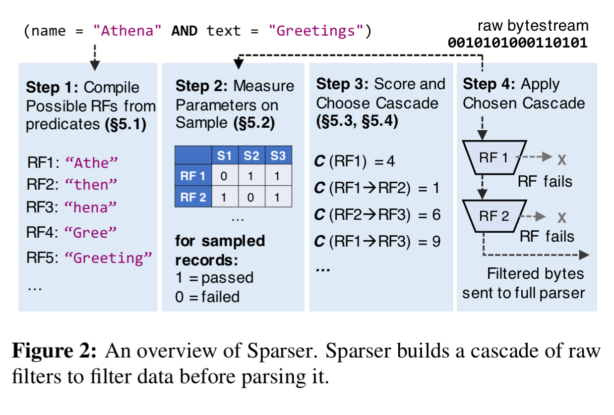
Sparser can make a big difference to execution times. Across a variety of workloads in the evaluation, Sparser achieved up to a 22x speed-up compared to Mison. This is a big deal, because serialising (and de-serialising) is a significant contributor to overall execution times in big data analytic workloads. So much so, that when integrated into a Spark system, end-to-end application performance improved by up to 9x.
Efficient raw filters
Raw filters (RF) operate over raw bytestreams and can produce false positives but no false negatives. They are designed to be SIMD efficient. There are two raw filter types: substring search and key-value search.
Say we have a predicate like this: name = "Athena" AND text = "My submission to VLDB". Substring search just looks for records that contain a substring sequence from the target values. For efficiency reasons it considers 2, 4, and 8-byte wide strings. Sticking with 4-byte substrings, we have several we could potentially use for matching, e.g. ‘Athe’, ‘ubmi’ or ‘VLDB’. Using VLDB as an example, the string is repeated eight times in a 32-byte vector register. We need 4 one-byte shifts to cover all possible matching positions in an input sequence:
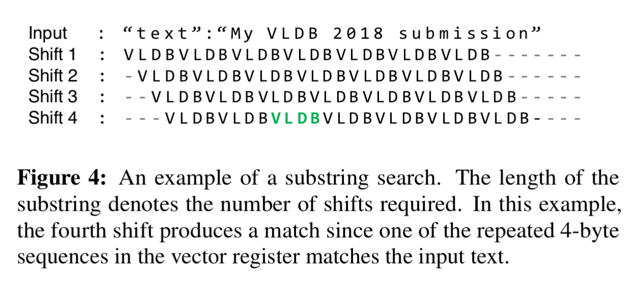
Note that the example in the figure above is actually a false positive for the input predicate. That’s ok. We don’t mind a few of those getting through.
The main advantage of the substring search RF is that, for a well-chosen sequence, the operator can reject inputs at nearly the speed of streaming data through a CPU core.
Key-value search looks for all co-occurrences of a key and a corresponding value within a record. The operator takes three parameters: a key, a value, and a set of one-byte delimiters (e.g. ,). After finding an occurrence of the key, the operator searches for the value and stops searching at the first occurring delimiter character. The key, value, and stopping point can all be searched for using the packed vector technique we looked at for substrings.
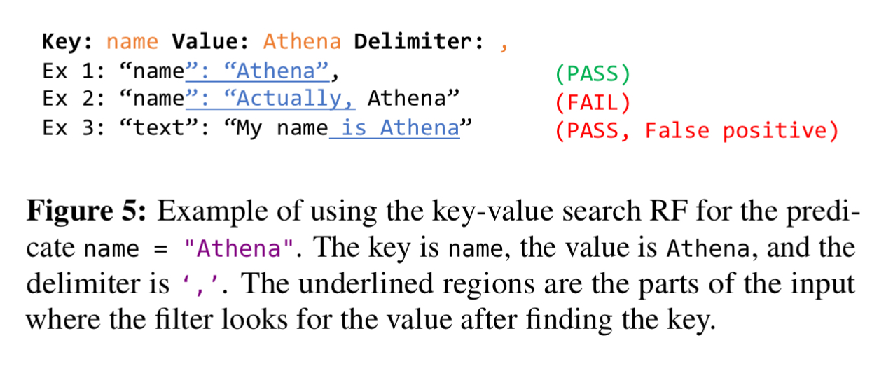
Whereas substring searches support both equality and LIKE, key-value filters do not support LIKE. This prevents false negatives from getting through.
Optimising filter cascades
Sticking with the example predicate name = "Athena" AND text = "My submission to VLDB", there are multiple raw filters we could consider, and multiple ways to order those filters. For example, if “VLDB” is highly selective it might be good to run a substring filter on VLDB first, and then feed the results into a key-value filter looking for name = "Athena". But if ‘VLDB’ occurs frequently in the dataset, we might be better off doing the key-value filtering first, and the substring search second. Or maybe we should try alternative substring searches in combination or instead, e.g. ‘submissi’. The optimum arrangement of filters in an RF cascade depends on the underlying data, the performance cost of running the individual raw filters, and their selectivity. We also have to contend with predicates such as(name = "Athena" AND text = "Greetings") OR name = "Jupiter", which are converted into DNF form before processing.
The first stage in the process is to compile a set of candidate RFs to consider based on clauses in the input query. Each simple predicate component of a predicate in DNF form is turned into substring and key-value RFs as appropriate. A substring RF is produced for each 4- and 8-byte substring of each token in the predicate expression, plus one searching for the token in its entirety . Key-value RFs will be generated for JSON, but for formats such as Avro and Parquet where the key name is unlikely to be present in the binary stream these are skipped. For the simple predicate name = "Athena" we end up with e.g.:
AthethenhenaAthena- key =
name, value =Athena, delimeters =,
Since these can only produce false positives, if any of these RFs fails, the record can’t match. For conjunctive clauses, we can simply take the union of all the simple predicate RFs in the clause. If any of them fail, the record can’t match. For disjunctions (DNF is the disjunction of conjunctions) then we require that an RF from each conjunction must fail in order to prevent false negatives.
Now Sparser draws a sample of records from the input and executes (independently) all of the RFs generated in the first step. It stores the passthrough rates of each RF in a compact matrix structure as well as recording the runtime costs of each RF and the runtime cost for the full parser.
After sampling, the optimizer has a populated matrix representing the records in the sample that passed for each RF, the average running time of each RF, and the average running time of the full parser.
Next up to 32 possible candidate RF cascades are generated. A cascade is a binary tree where non-leaf nodes are RFs and leaf nodes are decisions (parse or discard). Sparser generates trees up to depth D = 4. If there are more than 32 possible trees, then 32 are selected at random by picking a random RF generated from each token in round-robin fashion.
Now Sparser estimates the costs of the candidate cascades using the matrix it populated during the sampling step. Since the matrix stores a results of each pass/fail for an RF as single bit in the matrix, the passthrough rate of RF i is simply the number of 1’s in the ith row of the matrix. The joint passthrough rate of any two RFs is the bitwise and of their respective rows.
The key advantage to this approach is that these bitwise operations have SIMD support in modern hardware and complete in 1-3 cycles on 256-bit values on modern CPUs (roughly 1ns on a 3GHz processor).
Using this bit-matrix technique, the optimiser adds at most 1.2% overhead in the benchmark queries, including the time for sampling and scoring.
Periodic resampling
Sparser periodically recalibrates the cascade to account for data skew or sorting in the underlying input file. Consider an RF that filters by date and an input file sorted by date – it will either be highly selective or not selective at all depending on the portion of the file currently being processed.
Sparser maintains an exponentially weighted moving average of its own parsing throughput. In our implementation, we update this average on every 100MB block of input data. If the average throughput deviates significantly (e.g. 20% in our implementation), Sparser reruns its optimizer to select a new RF cascade.
Experimental results
Sparser is implemented in roughly 4000 lines of C, and supports mapping query predicates for text logs, JSON, Avro, Parquet, and PCAP. The team also integrated Sparser with Spark using the Data Sources API. Sparser is evaluated across a variety of workloads, datasets, and data formats.
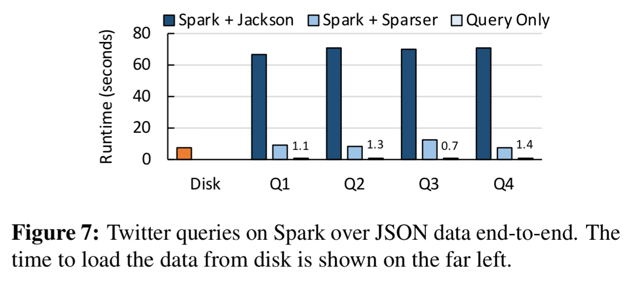
Here you can see the end-to-end improvements when processing 68GB of JSON tweets using Spark:
Avro and Parquet formats get a big boost too:
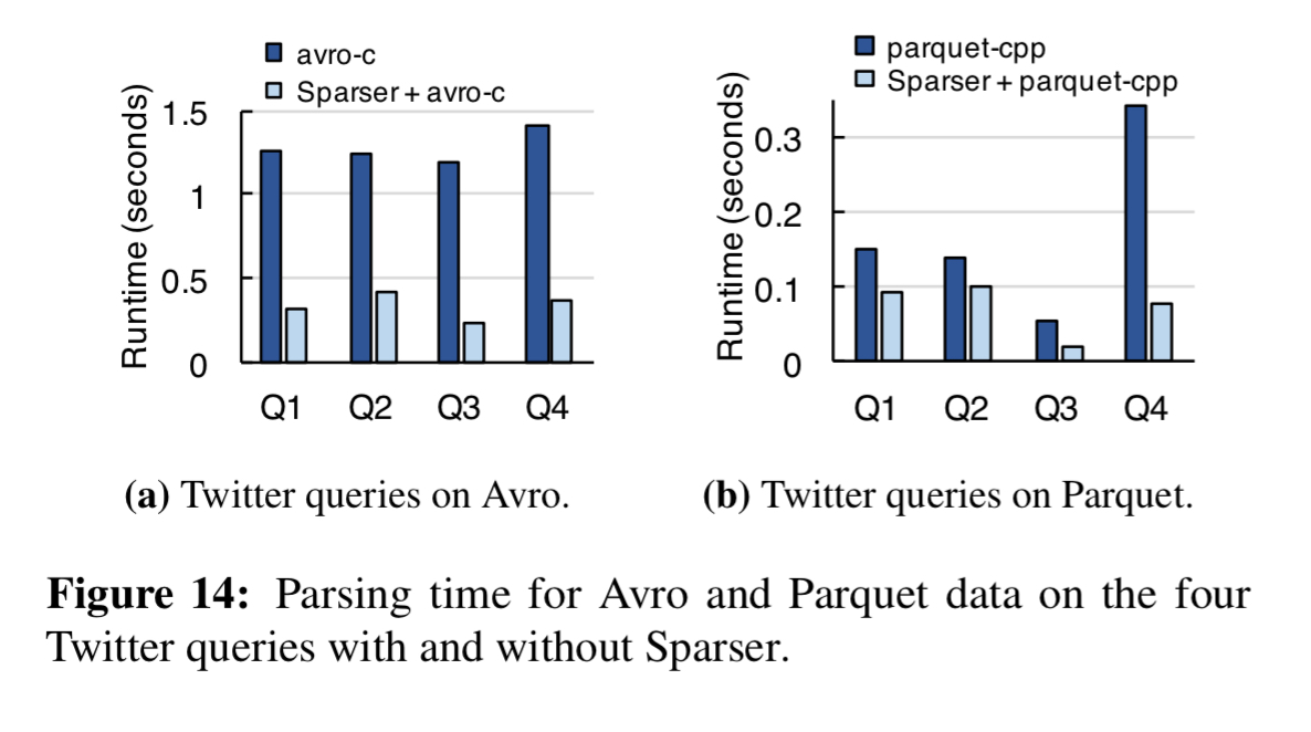
I’m short on space to cover the evaluation in detail, but here are the highlights:
- With raw filtering, Sparser improves on state-of-the-art JSON parsers by up to 22x. For distributed workloads it improves the end-to-end time by up to 9x.
- Parsing of binary formats such as Avro and Parquet are accelerated by up to 5x. For queries over unstructured text logs, Sparser reduces the runtime by up to 4x.
- Sparser selects RF cascades that are within 10% of the global optimum while incurring only a 1.2% runtime overhead.
In a periodic resampling just using a date based predicate, the resampling and re-optimisation process improved throughput by 25x compared to a sticking with the initially selected RF cascade for the whole job.
See the blog post from the authors and a link to the code here.
There’s a typo on your first quote: “2GMB/s” should be “2GB/s”.