Optimus: an efficient dynamic resource scheduler for deep learning clusters Peng et al., EuroSys’18
(If you don’t have ACM Digital Library access, the paper can be accessed either by following the link above directly from The Morning Paper blog site).
It’s another paper promising to reduce your deep learning training times today. But instead of improving the programming model and/or dataflow engine, Optimus improves the scheduling of jobs within a cluster. You can run it on top of Kubernetes, and the authors claim about a 1.6x reduction in makespan compared to the mostly widely used schedulers today.
Deep learning clusters
We’re using ever larger models, with ever increasing amounts of data (at least, whenever we can get our hands on it). In general this improves the learning accuracy, but it also increases the training time. The most common approach is parallel training using a machine learning cluster. Typically a model is partitioned among multiple parameter servers, and training data is spread across multiple workers. Workers compute parameter updates and push them to the respective parameter server.
Training is an iterative process with a dataset divided into chunks, and each chunk further divided into mini-batches. A training step processes one mini-batch and updates gradients (parameter values). We can also compute a training performance metric at the end of each mini-batch. When all mini-batches have been processed, that completes one epoch. Typically a model is trained for many epochs (tens to hundreds) until it converges (the performance metric stabilises).
The following chart shows example performance metrics and their progress over epochs:
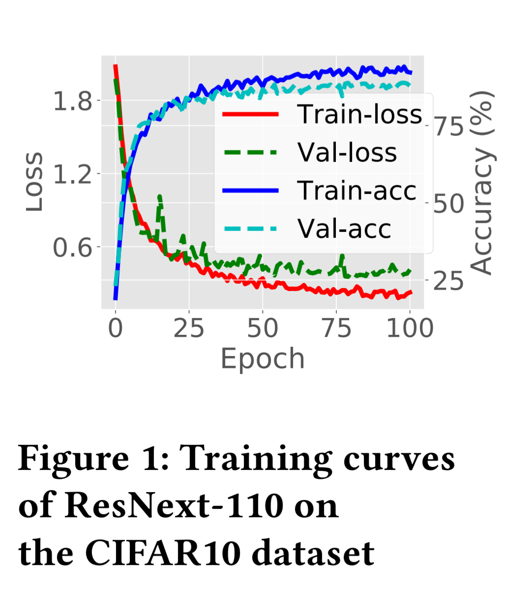
Training may be synchronous (a barrier at the end of each training step), or asynchronous.
…different from experimental models, production models are mature and can typically converge to the global/local optimum very well since all hyper-parameters (e.g., learning rate – how quickly a DNN adjusts itself, mini-batch size) have been well-tuned during the experimental phase. In this work, we focus on such production models, and leverage their convergence property to estimate a training job’s progress towards convergence.
In particular, Optimus uses the convergence of training loss.
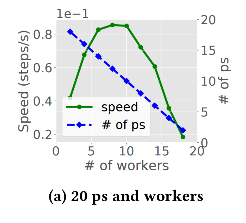
Cluster schedulers are used to allocate resources to parameter servers and workers. Existing schedulers such as Borg and YARN allocate a fixed amount of resource to each job upon its submission, and do not vary resource while a job is running. The number of allocated workers and parameter servers influence training speed. Suppose we have a budget of 20 containers, that we can divide up as we see fit between parameter servers and workers. The following chart shows that for a ResNet-50 model, the maximal training speed is achieved with 8 workers and 12 parameter servers:
Alternatively, if we fix the ratio of parameter servers to workers at 1:1, and increase the number of containers available while maintaining that ratio, we get a chart like this:
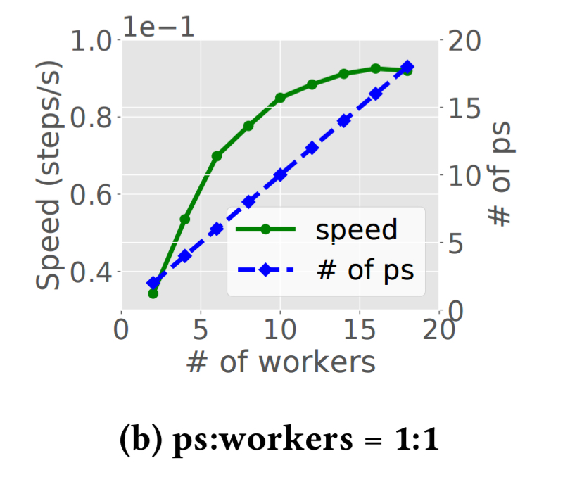
Notice that beyond a certain point, adding more resources starts to slow down training! Overall training times can vary from minutes to weeks depending on the model and data.
Optimus high-level design
In a production cluster, job training speed is further influenced by many runtime factors, such as available bandwidth at the time. Configuring a fixed number of workers/parameter servers upon job submission is hence unfavorable. in Optimus, we maximally exploit varying runtime resource availability by adjusting numbers and placement of workers and parameter servers, aiming to pursue the best resource efficiency and training speed at each time.
To make good decisions, Optimus needs to understand the relationship between resource configuration and the time a training job takes to achieve convergence. Optimus builds and fits performance models to estimate how many steps/epochs a job will need to reach convergence, and how different combinations of resource and parameter servers impact training speed. It takes about 10 samples to learn a good enough initial approximation.
… we run a job for a few steps with different resource configurations, learn the training speed as a function of resource configurations using data collected from these steps, and then keep tuning our model on the go.
Using the predictions obtained from these models, Optimus allocates resources to workers and parameter servers using a greedy algorithm based on estimated marginal gains. Tasked are then placed using the smallest number of servers possible, subject to the following constraint: each server runs p parameter servers, and w workers (i.e., the values of p and w are the same across all servers).
Modeling deep learning jobs
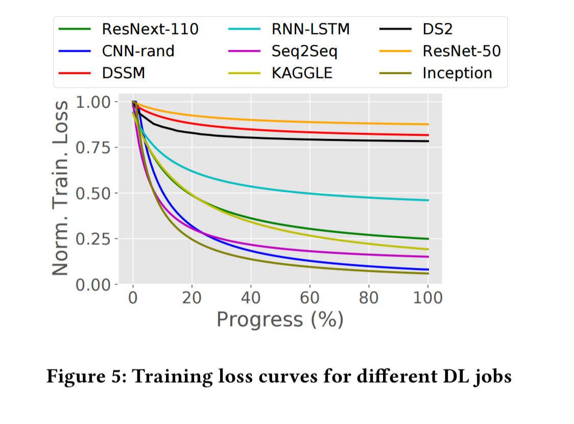
The first model is used to estimate the number of steps/epochs a job needs to reach completion. SGD converges at a rate of O(1/k) given number of steps k. So we can approximate the training loss curve using the following model:

Where l is the training loss and 
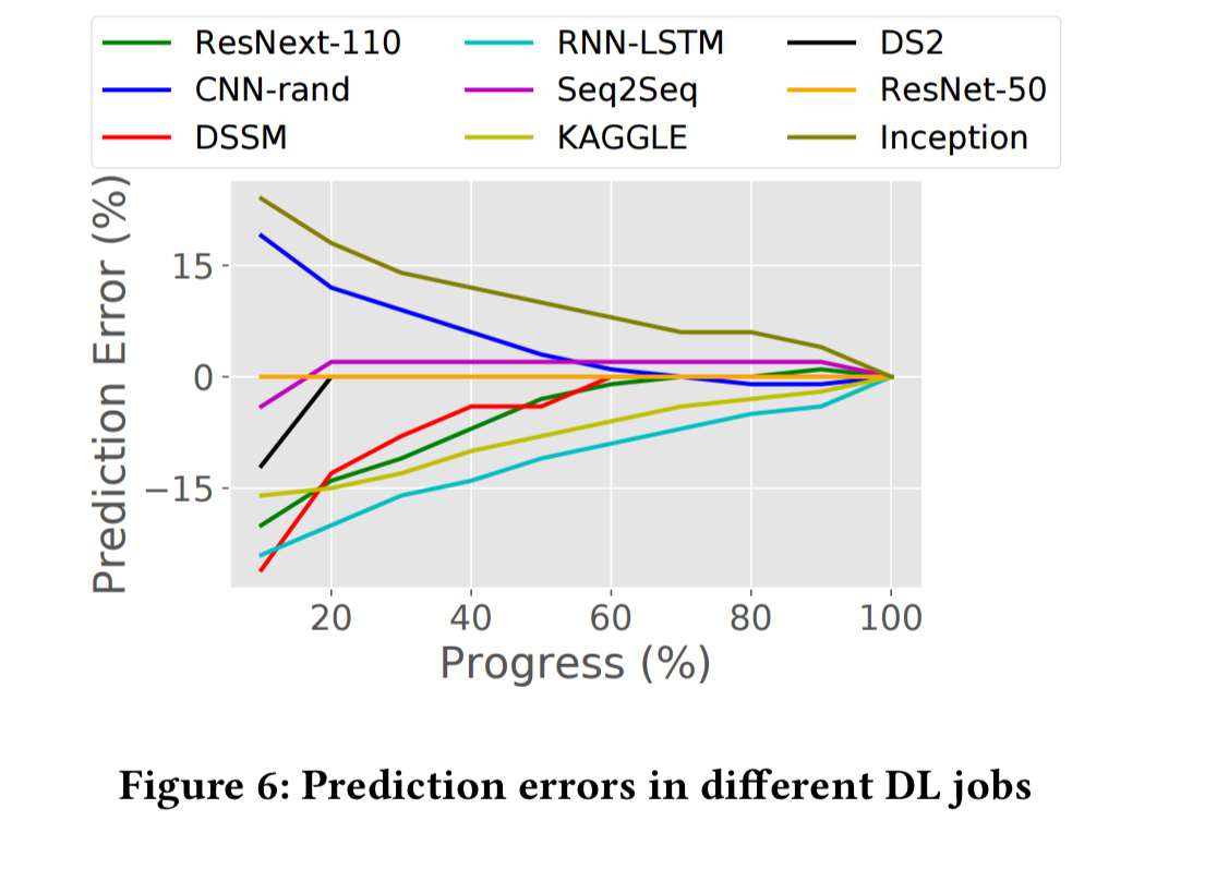
As we get more data points after each step, the model fit (prediction error) improves, as shown below:
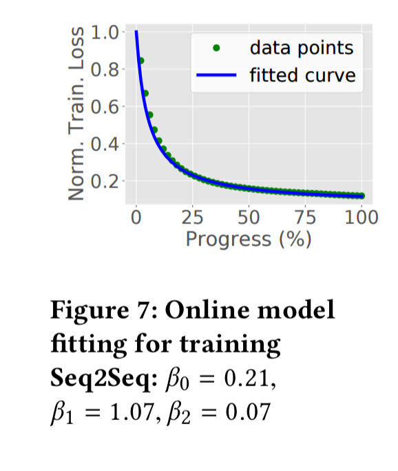
Here’s an example of model fitting when training a Seq2Seq model:
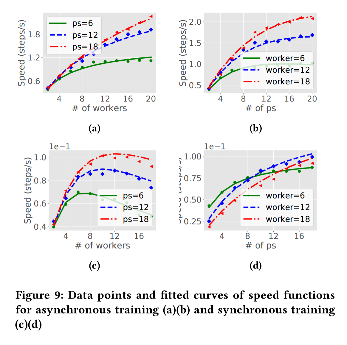
The second model is used to estimate training speed based on the computation and communication patterns of different parameter server and worker configurations. Let’s start with asynchronous training, where workers process mini-batches at their own pace. Assuming w workers and p parameter servers the training speed function f(p,w) can be approximated as follows:

With synchronous training we progress is determined by the dataset size M, meaning that each worker is allocated 

To learn the values of the 
Dynamic scheduling
Jobs arrive in an online manner, and at each time step Optimus allocates resources to newly submitted jobs, and adjusts the resource allocations of existing jobs. The scheduler aims to minimize the average completion time of these jobs. With knowledge of the estimated number of training steps remaining, and a model of how training speed is impacted by resources, this becomes a constraint solving problem. The authors introduce a notion of marginal gain as a heuristic leading to an efficient approximation. Let the dominant resource in the cluster be the resource type that is most contended (at least that’s my reading, the actual paper says “has maximal share in the overall capacity of the cluster”, and I’m not 100% certain what the authors mean by that). The marginal gain is the estimated reduction in job completion time when one worker (or parameter server) is added to a job, divided by the amount of the dominant resource that a worker (parameter server) occupies.
Initially each job is allocated one worker and one parameter server. Then we iterate, greedily adding a worker (parameter server) to the job with the largest marginal gain in each iteration. Iteration stops when cluster resource is exhausted, or the marginal gains are all negative.
Now we have an allocation of workers and parameter servers to each job, the next stage is to place them across servers.
Given the numbers of workers and parameter servers in a synchronous training job, the optimal worker/parameter server placement principle to achieve the maximal training speed for the job, in a cluster of homogeneous servers, is to use the smallest number of servers to host the job, such that the same number of parameter servers and the same number of workers are deployed on each of these servers.
It’s also important to detect stragglers and replace them by launching a new worker.
The final piece of the puzzle is ensuring a good workload balance among the parameter servers through careful division of the model parameters. Space precludes me from covering this here, but you’ll find a description in section 5.3 of the paper.
Evaluation
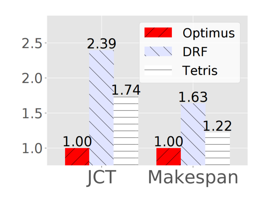
Optimus is compared against a fairness-based scheduler using Dominant Resource Fairness as used in many existing systems, as well as Tetris, which preferentially allocates resources to jobs with low duration or small resource consumption. Optimus reduces the average completion time and makespan by 2.39x and 1.63x respectively as compared to the DRF based scheduler.
The resource allocation algorithm is the biggest contributing factor to the improvements. Optimus can schedule 100,000 tasks on 16,000 nodes in about 5 seconds.
Our experiments on a Kubernetes cluster show that Optimus outperforms representative cluster schedulers significantly.
