Learning transferable architectures for scalable image recognition Zoph et al., arXiv 2017
Things move fast in the world of deep learning! It was only a few months ago that we looked at ‘Neural architecture search with reinforcement learning.’ In that paper, Zoph et al., demonstrate that just like we once designed features by hand but later found better results by learning them, we can get state-of-art results by learning model architectures too (as opposed to hand-designing them). One of the drawbacks of learning an architecture is that each experiment requires training a model, so it’s computationally very expensive overall. Just a few months on, and Zoph et al., are back with an update in which they show how to significantly reduce the search time (e.g., from 4 weeks to 4 days on CIFAR-10), and how architectures learned on smaller problem sets (e.g. CIFAR-10) can be successfully transferred to larger ones (e.g. ImageNet). The combination opens the door to using learned components / architectures on large-scale problems.
Don’t get me wrong, we’re still talking about needing a lot of compute power – a pool of 450 GPUs sampled 20,000 child models and then fully trained the top 250 to determine the very best architecture for CIFAR-10. However, this is a big step forward in what still seems to me to be an inevitable direction – learning better building blocks for constructing models. The key results of the paper are certainly impressive:
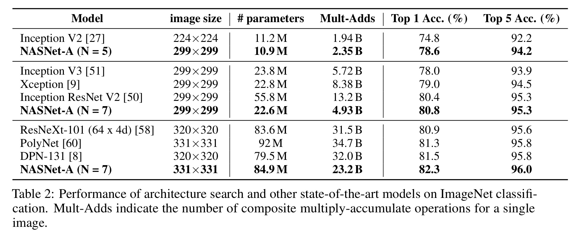
- Taking the best convolutional cell design learned on CIFAR-10, the authors transplant this cell into an ImageNet model and achieve state-of-the-art accuracy of 82.3% top-1 and 96.0% top-5. This is 0.8% better in top-1 accuracy than the best human-invented architectures while requiring 9 billion fewer FLOPS!
- Furthermore, at a comparable model size (approx 3 million parameters), a scaled down version suitable for mobile platforms achieves state-of-art results using only one-third of the training time.
Will the human expert frontier move from designing learning systems to designing meta-learning systems?
Our results have strong implications for transfer learning and meta-learning as this is the first work to demonstrate state-of-the-art results using meta-learning on a large scale problem. This work also highlights that learned elements of network architectures, beyond model weights, can transfer across datasets.
The new approach described in this paper builds on top of Neural Architecture Search, check out my earlier write-up on that for a quick refresher – I’ll include just the bare essentials below.
Designing a search space for Neural Architecture Search – architecture
In Neural Architecture Search (NAS), an RNN controller samples architectures from a search space, trains the resulting networks to convergence, and uses their efficacy to update the controller and refine the search.
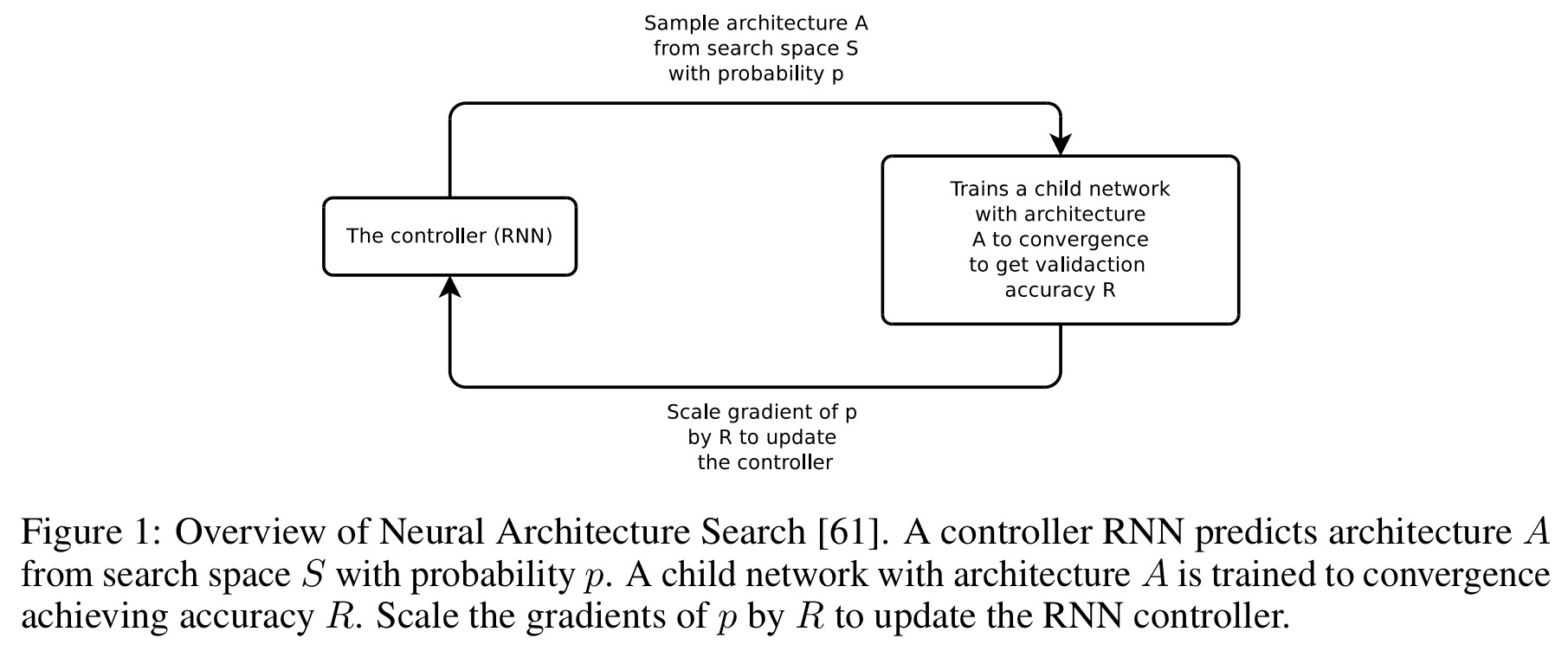
A key element of NAS is to design the search space S to generalize across problems of varying complexity and spatial scales. We observed that applying NAS directly on the ImageNet dataset would be very expensive and require months to complete an experiment. However, if the search space is properly constructed, architectural elements can transfer across datasets.
The team observed (and you’ll certainly recognise this if you sample enough papers), that successful CNNs often use repeated combinations of more elementary components and careful management of connections. So what if constrain the search to finding a good convolutional cell design, and simply stack it to handle inputs of arbitrary spatial dimensions and filter depth?
Actually, it turns out we need two convolutional cell designs: a design for a Normal Cell, which returns a feature map of the same dimension as its input; and a design for a Reduction Cell which reduces the feature map height and width by a factor of two.
Then for CIFAR-10 and ImageNet we might stack these cells together as so:
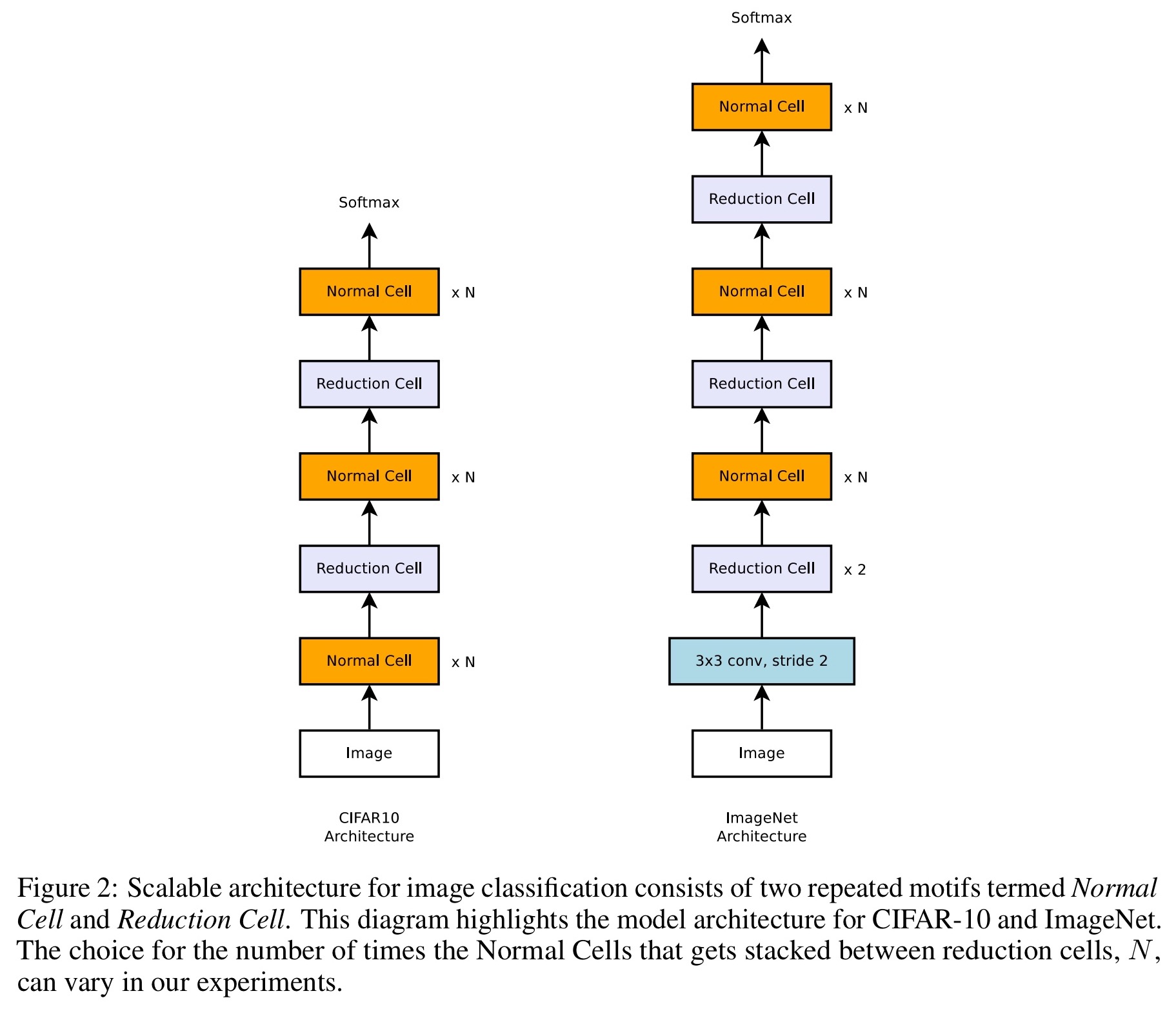
Thus compared to the original Neural Architecture Search which needs to predict the entire architecture, we have fixed the superstructure of the architecture and just need to predict the structures of the two cells used within it.
Designing a search space for Neural Architecture Search – convolutional cells
If this were Sesame Street, today’s programme would be brought to you by the number ‘5’.
Each cell is constructed of B = 5 blocks, receiving as input the outputs of the previous two lower layers (or the input image). Within each block, the controller makes 5 different prediction steps (5 decisions shaping the structure of the cell), using 5 distinct softmax classifiers. The choice of B=5 is a pragmatic one found to give good results, rather than the results of an exhaustive search.
Here’s the picture for one block (scribbled arrows mine):
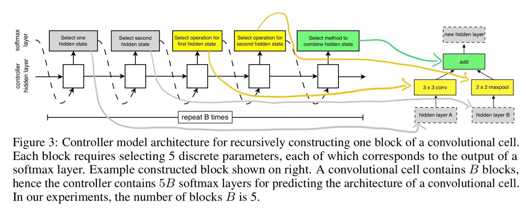
The five prediction steps are as follows:
- Select a first hidden state from h or from the set of hidden states created in previous blocks.
- Select a second hidden state from the same set of options as above.
- Select an operation to apply to the hidden state from step 1.
- Select an operation to apply to the hidden state in step 2.
- Select a method to combine the outputs from steps 3 and 4 to create a new hidden state. This can be either elementwise addition or concatenation along the filter dimension. All of the unused hidden states generated in the cell are concatenated together as well to provide the final cell output.
In steps 3 and 4, the operations are chosen from a menu of choices based on their prevalence in the CNN literature. These include:
- identity
- 1×3 then 3×1 convolution
- 1×7 then 7×1 convolution
- 3×3 average pooling
- 3×3, 5×5, and 7×7 max pooling
- 1×1 and 3×3 convolution
- 3×3 dilated convolation
- 3×3, 5×5, and 7×7 separable convolutions
To have the controller RNN predict both the Normal and Reduction cell we simply make the controller have 2 x 5B predictions in total, where the first 5B predictions are for the Normal Cell, and the second 5B predictions are for the Reduction Cell.
And the winner is…
Using a controller RNN trained using Proximal Policy Optimization with 20,000 child models sampled, the best performing cell designs turned out to look like this.
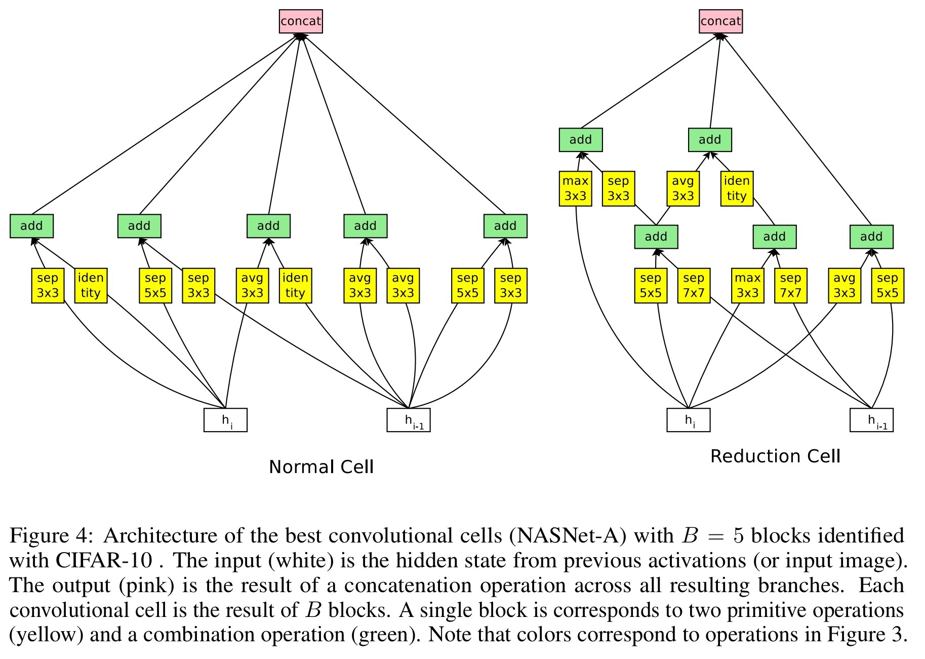
Note the higher-than-normal number of separable convolution operations.
After having learned the convolutional cell, several hyper-parameters may be explored to build a final network for a given task: (1) the number of cell repeats N, and (2) the number of filters in the initial convolutional cell. We employ a common heuristic to double the number of filters whenever the stride is 2.
Results on CIFAR-10
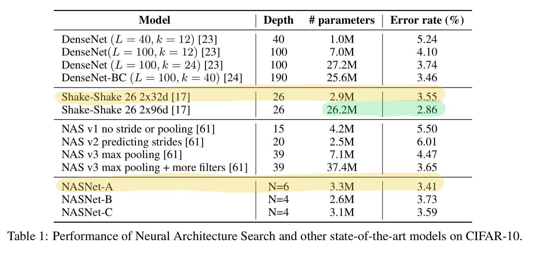
Setting N (number of cell repeats in a layer) to 4 or 6, and training for 600 epochs on CIFAR-10 using these cell designs (denoted NASNet-A in the table below) gives a state-of-the-art result for the model size. Only Shake-Shake 26 2x96d can beat it, and that uses an order of magnitude more parameters.
Results on ImageNet
Taking the same cells learned on CIFAR-10 and dropping them into ImageNet yields very interesting results.
… each model model based on the convolutional cell exceeds the predictive performance of the corresponding hand-designed model. Importantly, the largest model achieves a new state-of-the-art performance for ImageNet (82.3%) based on single, non-ensembled predictions, surpassing the previous state-of-the-art by 0.8%.
If you plot computational demand against number of parameters for top performing CNN architectures on ImageNet 2012 you can see that the learned cell structures dominate (red squares, line connecting them my own annotation).
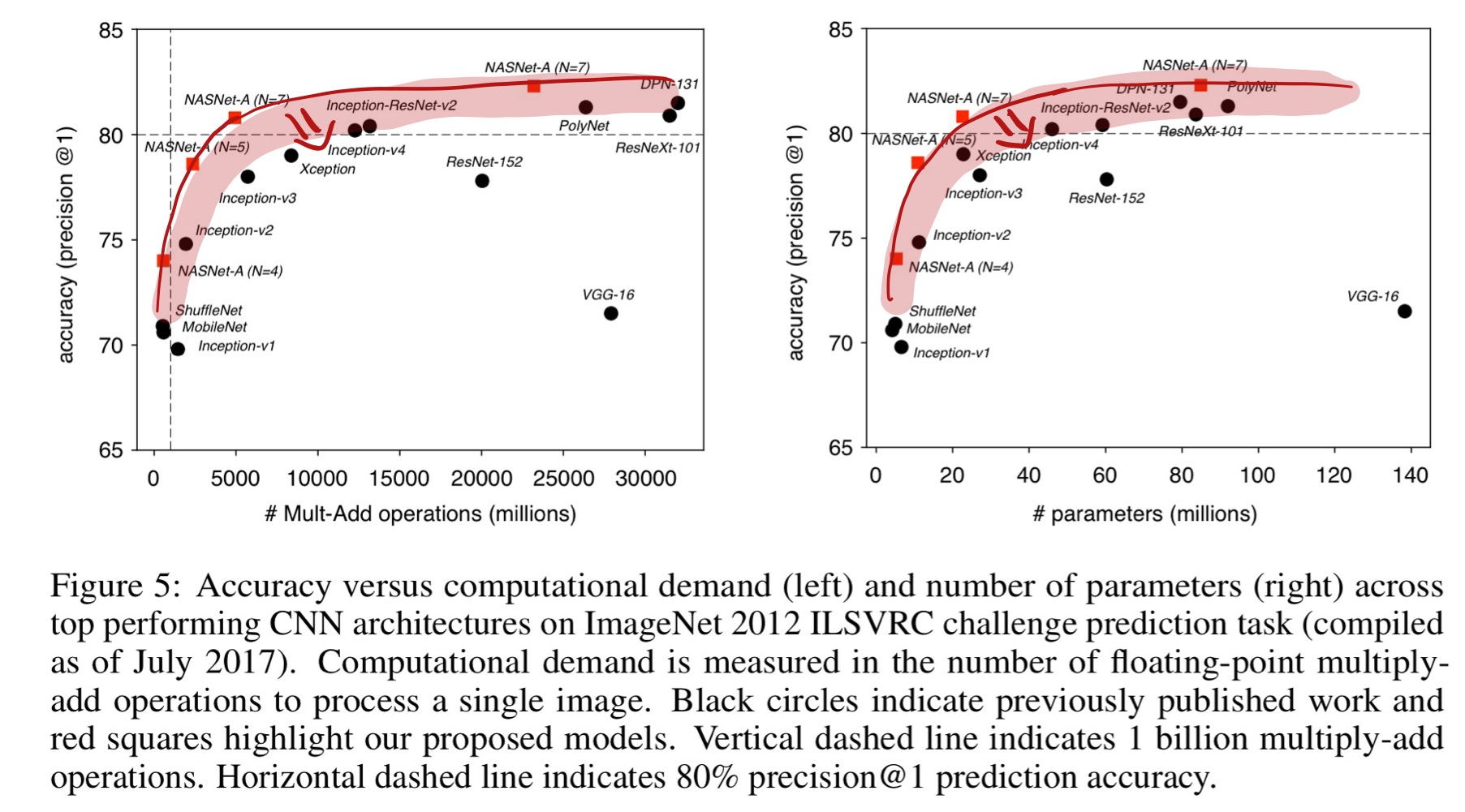
For ImageNet classification in resource-constrained settings (e.g., mobile), the learned cells surpass the previous state-of-the-art in accuracy using comparable computational demand.

In summary, we find that the learned convolutional cells are flexible across model scales achieving state-of-the-art performance across almost 2 orders of magnitude in computational budget.