DeepCoder: Learning to write programs Balog et al., ICLR 2017

I’m mostly trying to wait until the ICLR conference itself before diving into the papers to be presented there, but this particular paper follows nicely on from yesterday, so I’ve decided to bring it forward. In ‘Large scale evolution of image classifiers‘ we saw how it’s possible to learn a model for an image classification problem instead of trying to hand-engineer it. (Which incidentally paves the way for bootstrapping sophisticated ML systems the same way that we might bootstrap a compiler). But that’s a fairly constrained domain, surely the average programmer’s job is safe – we can’t learn to write any old program. Or can we? Well ok, no we can’t, but DeepCoder can learn how to solve simple programming tasks of the kind found in the most basic problems on programming competition websites. And it’s only going to get better!

Here’s an example:

This is the domain of Inductive Program Synthesis (IPS). DeepCoder is shown sets of inputs and outputs, and must learn a program that will produce the given outputs when presented with the given inputs (no memorization allowed!). Fundamentally this is a guided search across the space of all possible programs. To make that tractable we need to choose a language (a DSL) in which we’re going to express programs – using a general purpose language such as C++ yields far too big a search space. DeepCoder’s secret sauce is a neural network that is trained to predict the kinds of functions that might be useful when trying to recreate the outputs for a given set of inputs. Knowing the most likely functions the program will ultimately need to include guides the search and helps it find solutions much faster. The approach of integrating a learning module into an IPS system is called LIPS (Learning Inductive Program Synthesis).

The DeepCoding DSL

DeepCoding programs are simple sequences of function calls, the result of each call initialising a fresh variable that holds either a single integer or an integer array. The output of the program is the return value of the last function call.

The DSL contains the first-order functions head, last, take, drop, access, minimum, maximum, reverse, sort, and sum, and the higher-order functions map, filter, count, zipwith`, and `scanl. The pre-defined lambda functions which can be passed to these higher-order functions are:

• for map: (+1), (-1), (*2), (/2)2 (*(-1))2 (**2), (*3), (/3), (*4), (/4)
• for filter and count: (>0), (<0), (%2 == 0), (%2 == 1)
• for zipwith and scanl: (+), (-), (*), min, max

There’s is no explicit looping, but of course many of the provided functions do provide branching and looping internally.

The Learning Module

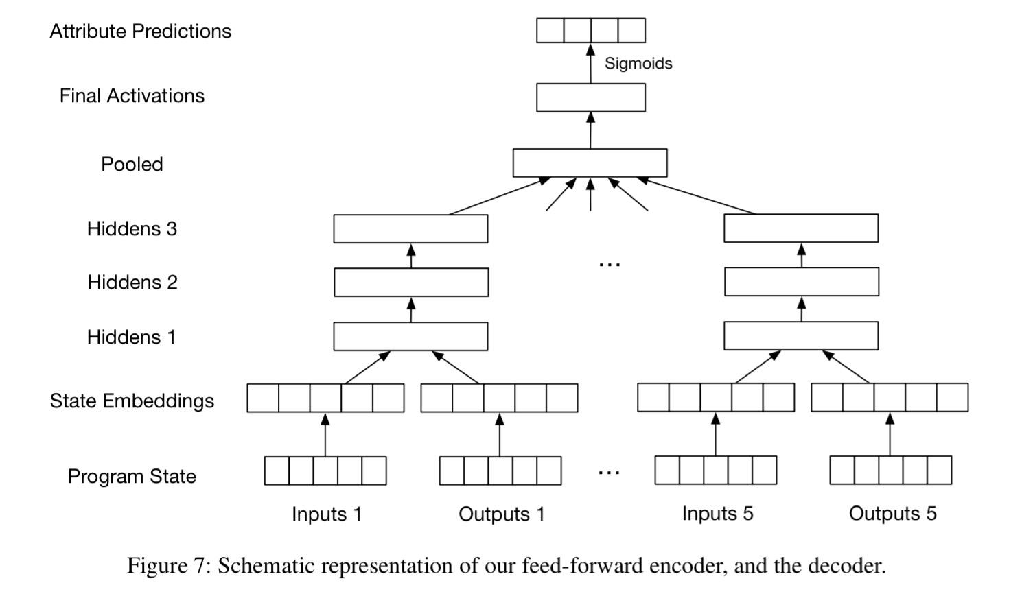
The learning module learns to predict the probability that each of the above functions is used in a given program, based on seeing an input-output pair. To take a simple example, given the input [3, 8, 1, 7] and the output [4, 12, 28, 32] the network should predict high probability for sort and (*4). The overall network structure looks like this:

With only three hidden layers, it’s actually a fairly simple structure compared to some of the models we looked at last week.

First, we represent the input and output types (singleton or array) by a one-hot-encoding, and we pad the inputs and outputs to a maximum length L with a special NULL value. Second, each integer in the inputs and in the output is mapped to a learned embedding vector of size E = 20. (The range of integers is restricted to a finite range and each embedding is parametrized individually.) Third, for each input-output example separately, we concatenate the embeddings of the input types, the inputs, the output type, and the output into a single (fixed-length) vector, and pass this vector through H = 3 hidden layers containing K = 256 sigmoid units each. The third hidden layer thus provides an encoding of each individual input-output example. Finally, for input-output examples in a set generated from the same program, we pool these representations together by simple arithmetic averaging.

To network outputs a log-unnormalised array of probabilities of each function appearing in the source code:

To generate training examples, DSL programs are enumerated, pruned to remove obvious issues such as redundant variables, or the existence of shorter equivalent programs (approximated by identical behaviour on a set of inputs). Valid inputs for a program are generated by putting a constraint on the output values and propagating this constraint backward through the program. Input-output pairs are then generated by picking inputs from the pre-computed valid ranges and executing the program to obtain the output values.

Searching for Solutions

At this point we have a set of inputs and outputs, and some clues as to which functions are most likely to be included in a program that generated those outputs. We know use this information to guide a search. The team evaluate a few different search strategies:

• Depth-first search (DFS) over programs of some maximum length T. When the search extends a partial program, it considers functions in probability order (highest probability first of course!).
• A sort and add scheme which maintains a set of active functions and performs DFS with the active function set only. When the search fails, the next most probable function (or set of functions) is added to the active set and the search restarts.
• Use of the Sketch SMT-based program synthesis tool, with a similar sort-and-add scheme used to guide its search
• Use of the program synthesis tool also using a sort-and-add scheme

Let’s generate some programs!

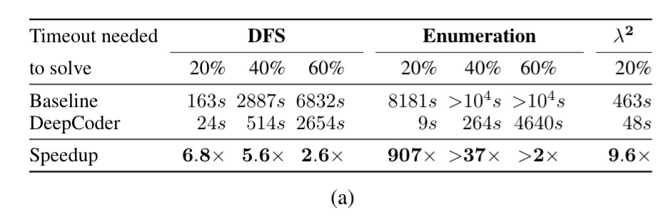
The main experiment looked at programs of length T=5 ( a search space on the order of 10¹⁰, supported by a neural network trained on programs of length T=4. The table below shows the results when trying to find 100 programs (Sketch is dropped from this part of the evaluation as it is significantly slower than the other methods).

The thing to remember when looking at the results is that there is no surprise that the search strategies can actually find successful programs. So what we’re really interested in is how long does it take to do so, and how much if any the learning component actually helps.

In the table above, the percentage columns tell you how long it took each variation to solve 20%, 40%, and 60% of the program generation challenges out of the 100 presented. The baseline row shows how long the search takes when given a function probability distribution that simply mirrors the global incidence of each function in the 500 program test set corpus. Thus the DeepCoder row is truly telling us what difference the neural network prediction make to search time.

We hypothesize that the substantially larger performance gains on Sort and add schemes as compared to gains on DFS can be explained by the fact that the choice of attribute function (predicting presence of functions anywhere in the program) and learning objective of the neural network are better matched to the Sort and add schemes.

Further experiments varying the length of the test programs (from 1 to 4 functions), and the length of the generated programs (from 1 to 5 functions) showed that the neural network can generalize to programs of different lengths than the programs in the training set.

Our empirical results show that for many programs, this technique [neural network guided search] improves the runtime of a wide range of IPS baselines by 1-3 orders. We have found several problems in real online programming challenges that can be solved with a program in our language, which validates the relevance of the class of problems that we have studied in this work. In sum, this suggests that we have made significant progress towards being able to solve programming competition problems, and the machine learning component plays an important role in making it tractable.

Of course, as the authors themselves point out, “there remain some limitations…“.