Having recovered somewhat from the last push on deep learning papers, it’s time this week to tackle the next batch of papers from the ‘top 100 awesome deep learning papers.’ Recall that the plan is to cover multiple papers per day, in a little less depth than usual per paper, to give you a broad sweep of what’s in them (See “An experiment with awesome deep learning papers“). You’ll find the first batch of papers in the archives starting from February 27th. For the next three days, we’ll be tackling the papers from the ‘convolutional neural network models’ section, starting with:
- ImageNet classification with deep convolutional neural networks, Krizhevsky et al., 2012
- Maxout networks, Goodfellow et al., 2013
- Network in network, Lin et al., 2013
- OverFeat: Integration recognition, localization and detection using convolutional networks, Sermanent et al., 2013
Ujjwal Karn’s excellent blog post “An intuitive explanation of convolutional neural networks” provides a some great background on how convolutional networks work if you need a refresher before diving into these papers.
ImageNet classification with deep convolutional neural networks
This is a highly influential paper that kicked off a whole stream of work using deep convolutional neural networks for image processing. Two factors changed that made this possible: firstly, the availability of large enough datasets (specifically, the introduction of ImageNet with millions of images, whereas the previous largest datasets had ‘only’ tens of thousands; and secondly the development of powerful enough GPUs to efficiently train large networks.
What makes CNNs such a good fit for working with image data?
Their capacity can be controlled by varying their depth and breadth, and they also make strong and mostly correct assumptions about the nature of images (namely, stationarity of statistics and locality of pixel dependencies). Thus, compared to standard feedforward neural networks with similarly-sized layers, CNNs have much fewer connections and parameters and so they are easier to train, while their theoretically-best performance is likely to be only slightly worse.
The network that Krizhevsky et al. constructed has eight learned layers – five of them convolutional and three fully-connected. The output of the last layer is a 1000-way softmax which produces a distribution over the 1000 class labels (the ImageNet challenge is to create a classifier that can determine which object is in the image). Because the network is too large to fit in the memory of one GPU, training is split across two GPUs and the kernels of the 2nd, 4th, and 5th convolutional layers are connected only to those kernel maps in the previous layer which reside on the same GPU.
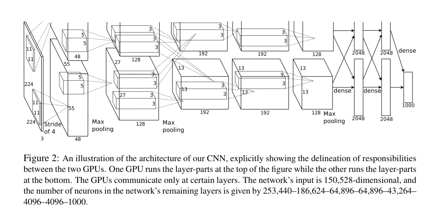
The authors single out four other aspects of the model architecture that they feel are particularly important:
- The use of ReLU activation (instead of
tanh). “Deep convolutional neural networks with ReLUs train several times faster than their equivalents with tanh units… Faster learning has a great influence on the performance of large models trained on large datasets“ - Using multiple GPUs (two!), and splitting the kernels between them with cross-GPU communication only in certain layers. The scheme reduces the top-1 and top-5 error rates by 1.7% and 1.2% respectively compared to a net with half as many kernels in each layer and trained on just one GPU.
- Using local response normalisation, which “implements a form of lateral inhibition inspired by the type found in real neurons, creating competition for big activities amongst neuron outputs computed using different kernels”.
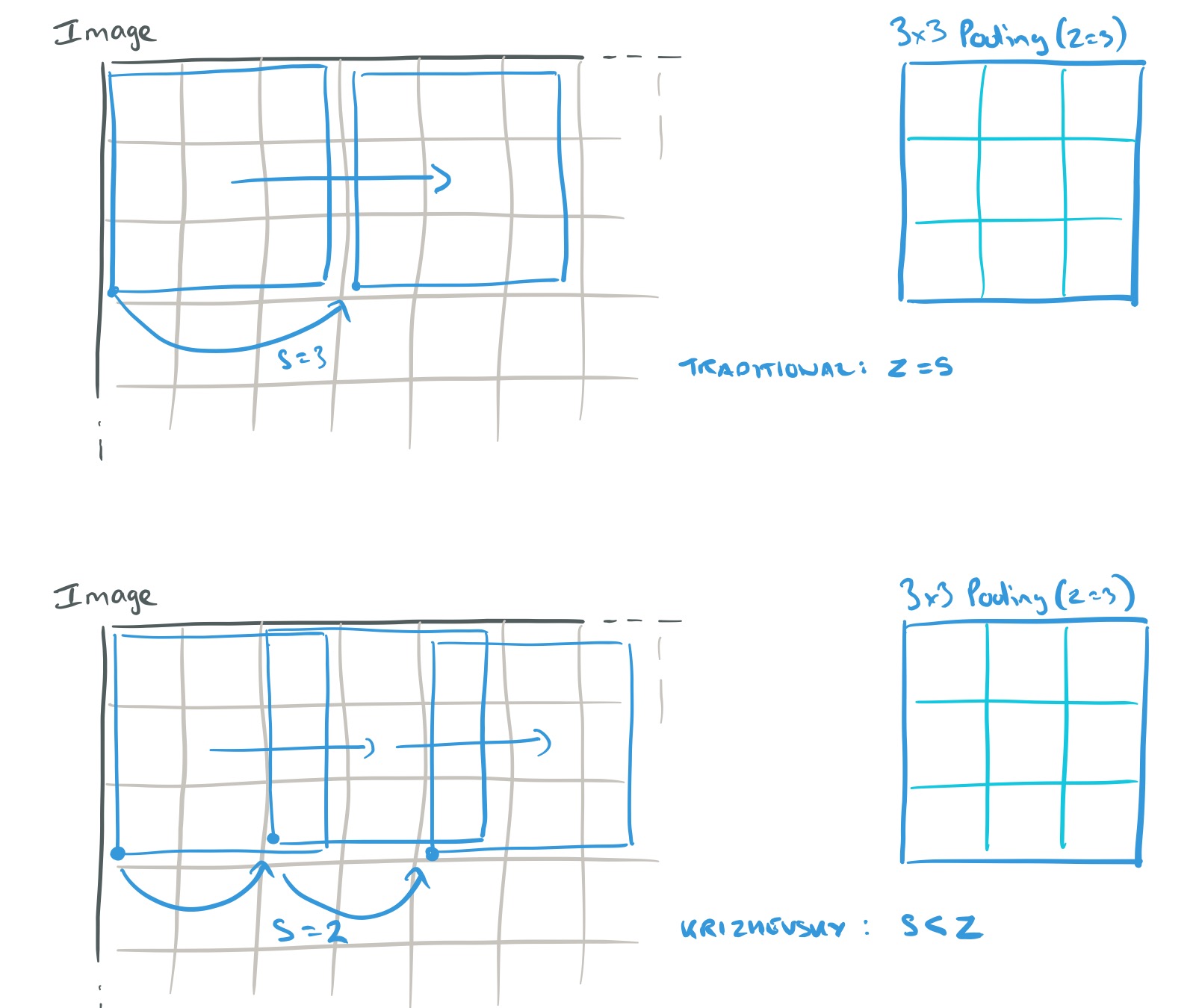
- Using overlapping pooling. Let pooling layers be of size z x z, and spaced s pixels apart. Traditionally pooling was used with s = z, so that there was no overlap between pools. Krizhevsky et al. used s = 2 and z = 3 to give overlapping pooling. This reduced the top-1 and top-5 error rates by 0.4% and 0.3% respectively.
To reduce overfitting dropout and data augmentation (translations, reflections, and principal component manipulation) is used during training.
The end result:
On ILSVRC-2010, our network achieves top-1 and top-5 test set error rates of 37.5% and 17.0%.
In ILSVRC-2012, the network achieved a top-5 test error rate of 15.3%, compared to 26.2% achieved by the second-best entry. That huge winning margin sparked the beginning of a revolution.
Our results show that a large, deep convolutional neural network is capable of achieving record-breaking results on a highly challenging dataset using purely supervised learning. It is notable that our network’s performance degrades if a single convolutional layer is removed. For example, removing any of the middle layers results in a loss of about 2% for the top-1 performance of the network. So the depth really is important for achieving our results.
For a more in-depth look at this paper, see my earlier write-up on The Morning Paper.
Maxout networks
Maxout networks are designed to work hand-in-glove with dropout. As you may recall, training with dropout is like training an exponential number of models all sharing the same parameters. Maxout networks are otherwise standard multilayer perceptron or deep CNNs that use a special activation function called the maxout unit. The output of a maxout unit is simply the maximum of its inputs.
In a convolutional network, a maxout feature map can be constructed by taking the maximum across k affine feature maps
(i.e., pool across channels, in addition spatial locations). When training with dropout, we perform the elementwise multiplication with the dropout mask immediately prior to the multiplication by the weights in all cases–we do not drop inputs to the max operator.
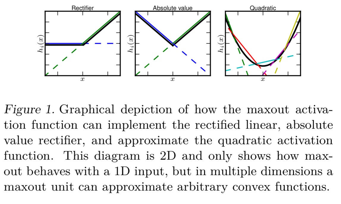
Maxout units make a piecewise linear approximation to an arbitrary convex function, as illustrated below.
Under evaluation, the combination of maxout and dropout achieved state of the art classification performance on MNIST, CIFAR-10, CIFAR-100, and SVHN (Street View House Numbers).
Why does it work so well? Dropout does exact model averaging in deeper architectures provided that they are locally linear among the space of inputs to each layer that are visited by applying different dropout masks…
We argue that dropout training encourages maxout units to have large linear regions around inputs that appear in the training data… Networks of linear operations and maxout may learn to exploit dropout’s approximate model averaging technique well.
In addition, rectifier units that saturate at zero are much more common with dropout training. A zero value stops the gradient from flowing through the unit making it hard to change under training and become active again.
Maxout does not suffer from this problem because gradient always flows through every maxout unit–even when a maxout unit is 0, this 0 is a function of the parameters and may be adjusted. Units that take on negative activations may be steered to become positive again later.
Network in Network
A traditional convolutional layer applies convolution by applying linear filters to the receptive field, followed by nonlinear activation. The outputs are called feature maps. In this paper Lin et al. point out that such a process cannot learn representations that distinguish well between non-linear concepts.
The convolution filter in CNN is a generalized linear model (GLM) for the underlying data patch, and we argue that the level of abstraction is low with GLM. By abstraction we mean that the feature is invariant to the variants of the same concept.
Even maxout networks impose the constraint that instances of a latent concept lie within a convex set in the input space, to which they make a piecewise linear approximation. A key question therefore, is whether or not input features do indeed require non-linear functions in order to best represent the concepts contained within them. The authors assert that they do:
…the data for the same concept often live on a nonlinear manifold, therefore the representations that capture these concepts are generally highly nonlinear function of the input. In NIN, the GLM is replaced with a ”micro network” structure which is a general nonlinear function approximator. In this work, we choose multilayer perceptron as the instantiation of the micro network, which is a universal function approximator and a neural network trainable by back-propagation.
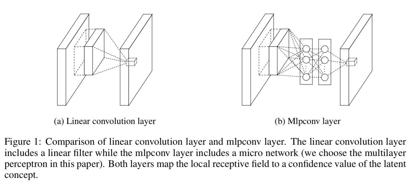
And that’s the big idea right there, replace the linear convolutional layer with a mini multilayer perceptron network (called an mlpconv layer). We know that such networks are good at learning functions, so let’s just allow the mlpconv network to learn what the best convolution function is. Since the mlpconv layers sit inside a larger network model, the overall approach is called “network in network.”
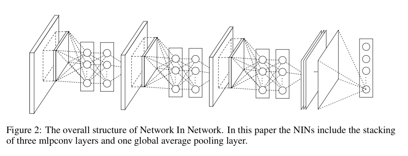
The second change that Lin et al. make to the traditional architecture comes at the last layer:
Instead of adopting the traditional fully connected layers for classification in CNN, we directly output the spatial average of the feature maps from the last mlpconv layer as the confidence of categories via a global average pooling layer, and then the resulting vector is fed into the softmax layer. In traditional CNN, it is difficult to interpret how the category level information from the objective cost layer is passed back to the previous convolution layer due to the fully connected layers which act as a black box in between. In contrast, global average pooling is more meaningful and interpretable as it enforces correspondance between feature maps and categories, which is made possible by a stronger local modeling using the micro network.
On CIFAR-10 (10 classes of natural images with 50,000 traning images in total, and 10,000 testing images), the authors beat the then state-of-the-art by more than one percent.
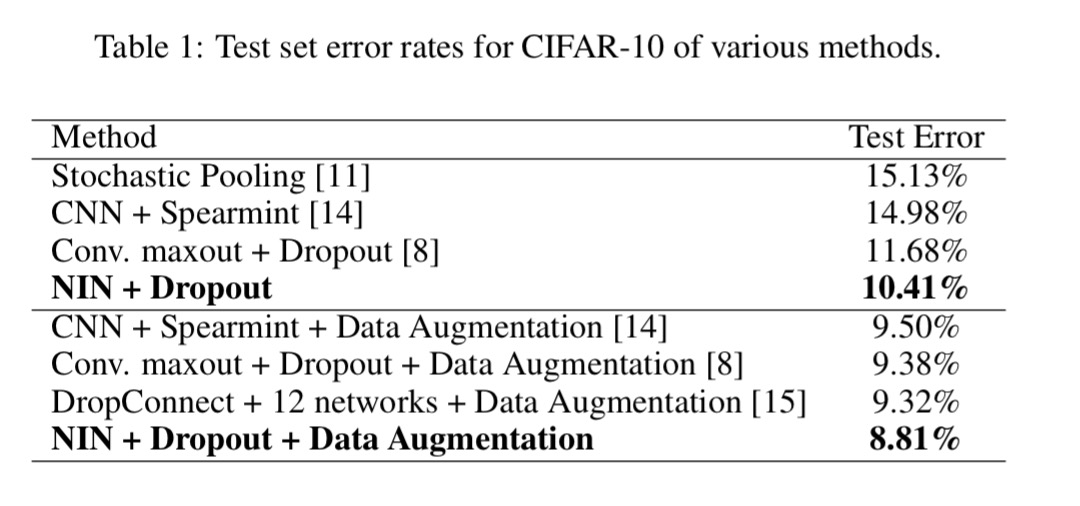
On CIFAR-100 they also beat the then best performance (without data augmentation, which was also not used to evaluate the N-in-N approach) by more than one percent. With the street view house numbers dataset, and with MNIST the authors get good results, but not quite state-of-the-art.
OverFeat: Integrated recognition, localization and detection using convolutional networks
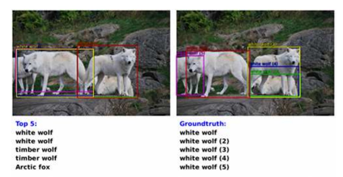
OverFeat shows how the features learned by a CNN-based classifier can also be used for localization and detection. On the ILSVRC 2013 dataset OverFeat ranked 4th in classification, 1st in localization, and 1st in detection. We know what the classification problem is (what object is in this image), but what about the localization and detection problems? Localization is like classification, but the network must also produce a bounding box showing the boundary of the detected object:
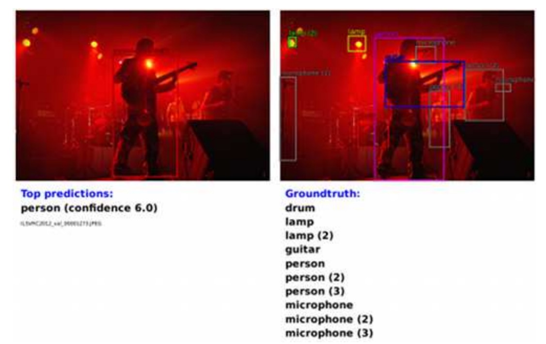
The detection problem involves images which may contain many small objects, and the network must detect each object and draw its bounding box:
The main point of this paper is to show that training a convolutional network to simultaneously classify, locate and detect objects in images can boost the classification accuracy and the detection and localization accuracy of all tasks. The paper proposes a new integrated approach to object detection, recognition, and localization with a single ConvNet. We also introduce a novel method for localization and detection by accumulating predicted bounding boxes.
There’s a lot of detail in the OverFeat paper that we don’t have space to cover, so if this work is of interest this paper is one where I definitely recommend going on to read the full thing.
Since objects of interest (especially in the later detection task) can vary significantly in size and position within the image, OverFeat applies a ConvNet at multiple locations within the image in a sliding window fashion, and at multiple scales. The system is then trained to produce a prediction of the location and size of the bounding box containing an object relative to the window. Evidence for each object category is accumulated at each location and size.
Starting with classification, the model is based on Krizhevsky et al. (our first paper today) in the first five layers, but no contrast normalisation is used, pooling regions are non-overlapping, and a smaller stride is used (2 instead of 4). Six different scales of input are used, resulting in unpooled layer 5 maps of varying resolution. These are then pooled and presented to the classifier.
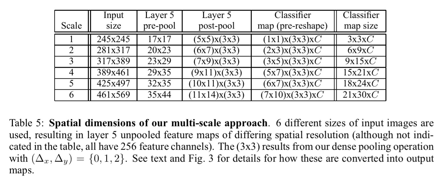
The following diagram summarises the classifier approach built on top of the layer 5 feature maps:
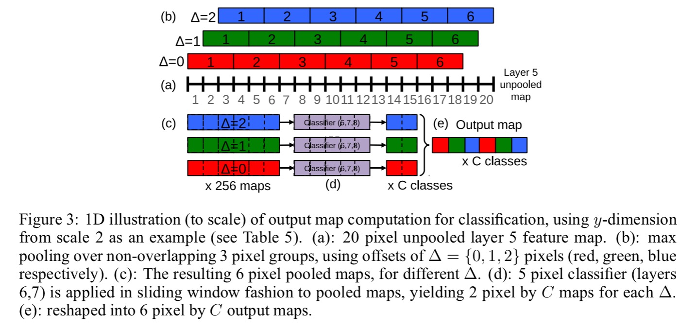
At an intuitive level, the two halves of the network — i.e. feature extraction layers (1-5) and classifier layers (6-output) — are used in opposite ways. In the feature extraction portion, the filters are convolved across the entire image in one pass. From a computational perspective, this is far more efficient than sliding a fixed-size feature extractor over the image and then aggregating the results from different locations. However, these principles are reversed for the classifier portion of the network. Here, we want to hunt for a fixed-size representation in the layer 5 feature maps across different positions and scales. Thus the classifier has a fixed-size 5×5 input and is exhaustively applied to the layer 5 maps. The exhaustive pooling scheme (with single pixel shifts (∆x, ∆y)) ensures that we can obtain fine alignment between the classifier and the representation of the object in the feature map.
Localization
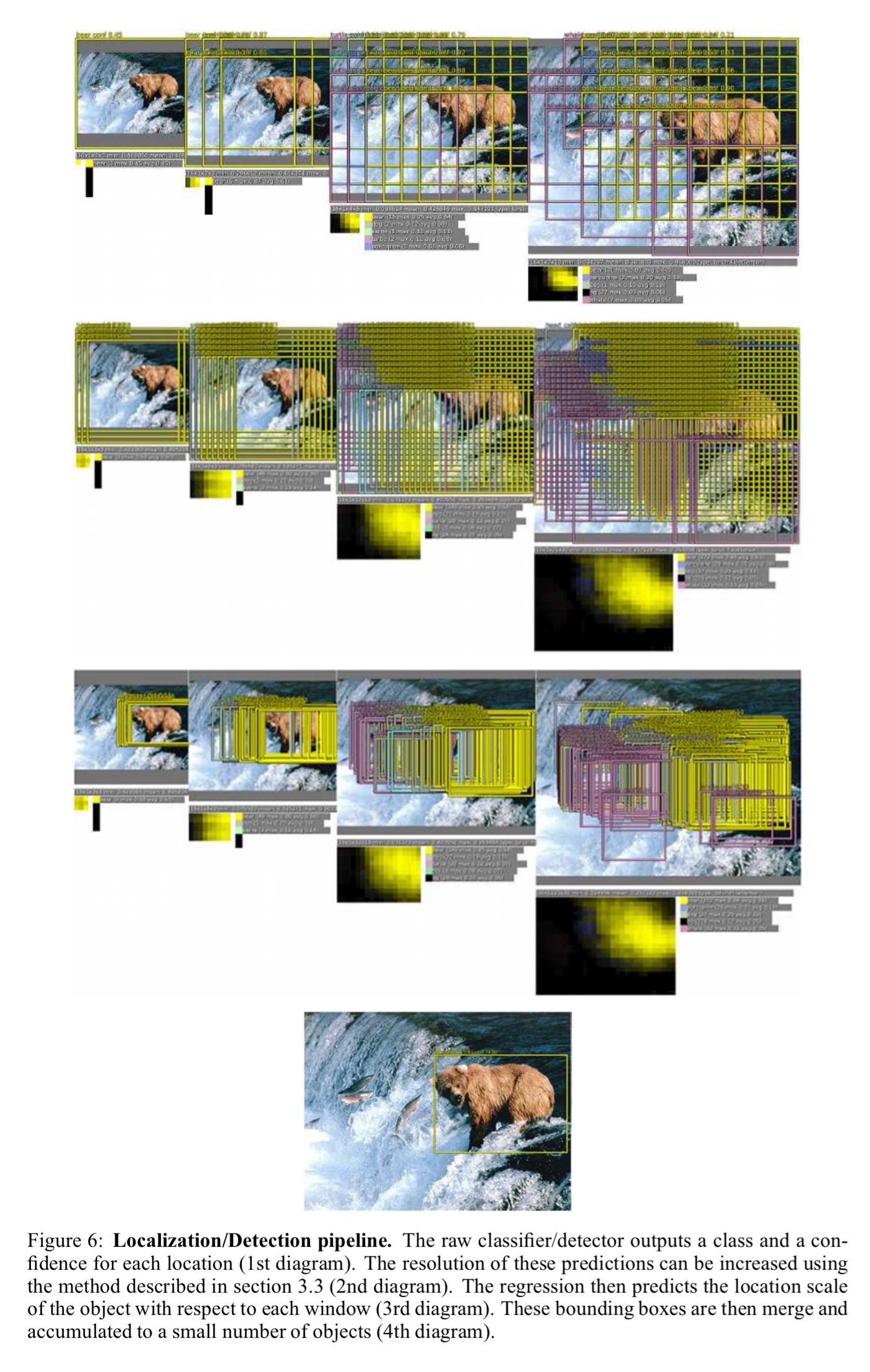
For localization the classifier layers are replaced by a regression networks trained to predict bounding boxes at each spatial location and scale. The regression predictions are then combined, along with the classification results at each location. Training with multiple scales ensure predictions match correctly across scales, and exponentially increases the confidence of the merged predictions.
Bounding boxes are combined based on the distance between their centres and the intersection of their areas, and the final prediction is made by taking the merged bounding boxes with maximum class scores. Figure 6 below gives a visual overview of the process:
Detection
Detection training is similar to classification training, but with the added necessity of predicting a background task when no object is present.
Traditionally, negative examples are initially taken at random for training, then the most offending negative errors are added to the training set in bootstrapping passes… we perform negative training on the fly, by selecting a few interesting negative examples per image such as random ones or most offending ones. This approach is more computationally expensive, but renders the procedure much simpler.
5 thoughts on “Convolutional neural networks, Part 1”
Comments are closed.