Today we’re looking at the ‘optimisation and training techniques’ section from the ‘top 100 awesome deep learning papers’ list.
- Random search for hyper-parameter optimization, Bergstra & Bengio 2012
- Improving neural networks by preventing co-adaptation of feature detectors, Hinton et al., 2012
- Dropout: a simple way to prevent neural networks from overfitting, Srivastava et al., 2014
- Adam: a method for stochastic optimization, Kingma & Ba, 2015
- Batch normalization: accelerating deep network training by reducing internal covariate shift, Ioffy & Szegedy, 2015
- Delving deep into rectifiers: surpassing human-level performance on ImageNet classification, He et al., 2015
Random search for hyper-parameter optimization
A machine learning model is itself parameterised by a large number of different parameters (e.g., learning rate, number of hidden units, strength of weight regularization). How you set these hyper-parameters can have a big impact on the overall results achieved, but finding an optimal set of hyper-parameters is far from easy. Essentially it boils down to picking some sets of parameters and trying them to see how well they work. How do you choose which sets to pick though? Even with a relatively small number of parameters it’s impossible to do an exhaustive search as the search space grows exponentially with the number of hyper-parameters. Furthermore, each trial is expensive – you have to train the full model using the hyper-parameters and see how well it performs, so practically you can’t do too many of them. In fact, it’s plain to see that you can only cover a tiny fraction of the overall search space.
Two common approaches for finding good hyper-parameter values as of 2012 were human intuition guided search, and a grid search in which you explore points in an evenly spaced grid laid over the search space.
A major drawback of manual search is the difficulty in reproducing results. This is important both for the progress of scientific research in machine learning as well as for ease of application of learning algorithms by non-expert users. On the other hand, grid search along does very poorly in practice (as discussed here).
What the authors show, is that a random search turns out to be a surprisingly effective technique, while also being just as easy to implement as a parallel search. The reason random search turns out to work so well is due to two key properties:
- It turns out that the parameter space has a low effective dimensionality . That is, some parameters matter much more than others when it comes to finding good settings.
- Which parameters those are varies according to the dataset (i.e., you can’t just find the two most important parameters for some model architecture and then always optimise based on just those).
If a researcher could know ahead of time which subspaces are important, then they could design an appropriate grid. But when they can’t know this, grid search fails. Consider the following simple illustration in 2-dimensional space. We have one parameter that turns out to be important (on the x-axis) and one that turns out to be unimportant (on the y-axis).
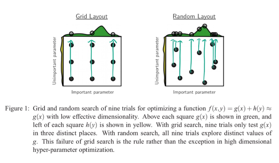
The grid search only touches three points along the important dimension, whereas the random search tests nine points – thus the random search has a much better chance of finding a good setting along this dimension.
To study the effects with real networks the authors plot random experiment efficiency curves, which look like this:
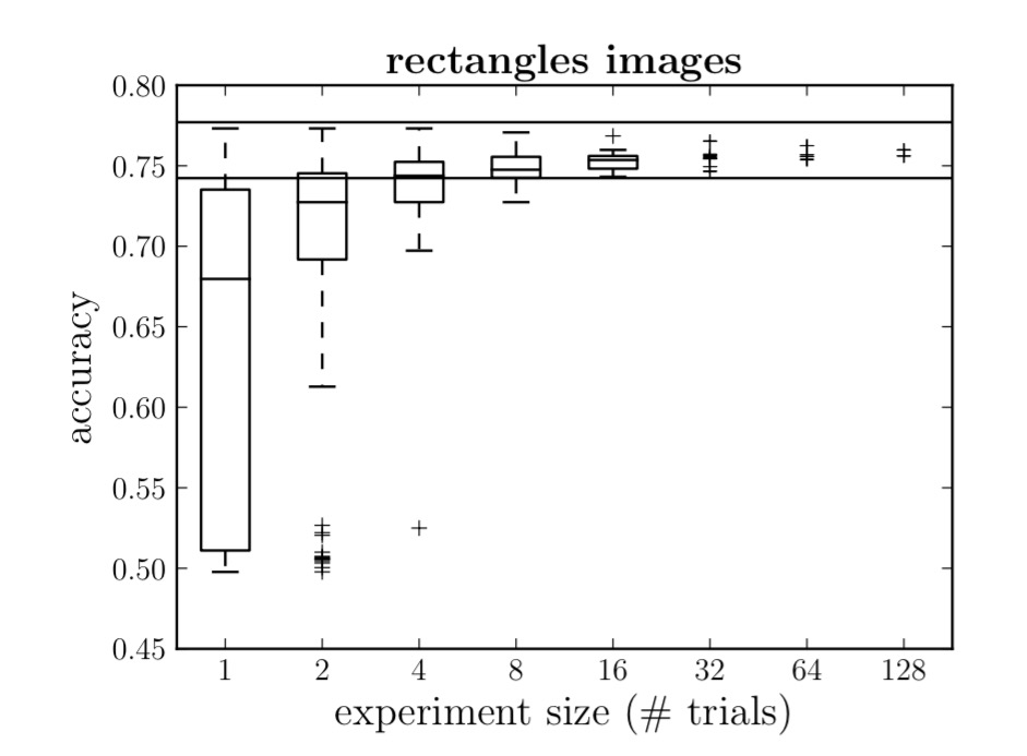
At each point x on the x-axis, you are seeing the results of exploring multiple hyper-parameter optimisation experiments, where each experiment trialled x different hyper-parameter sets. Thus on the y-axis we see the accuracy you could expect to achieve if running a hyper-parameter search with x trials.
There are two general trends in random experiment efficiency curves, such as the one in Figure 2: a sharp upward slope of the lower extremes as experiments grow, and a gentle downward slope of the upper extremes. The sharp upward slope occurs because when we take the maximum over larger subsets of the S trials, trials with poor performance are rarely the best within their subset. It is natural that larger experiments find trials with better scores. The shape of this curve indicates the frequency of good models under random search, and quantifies the relative volumes (in search space) of the various levels of performance.
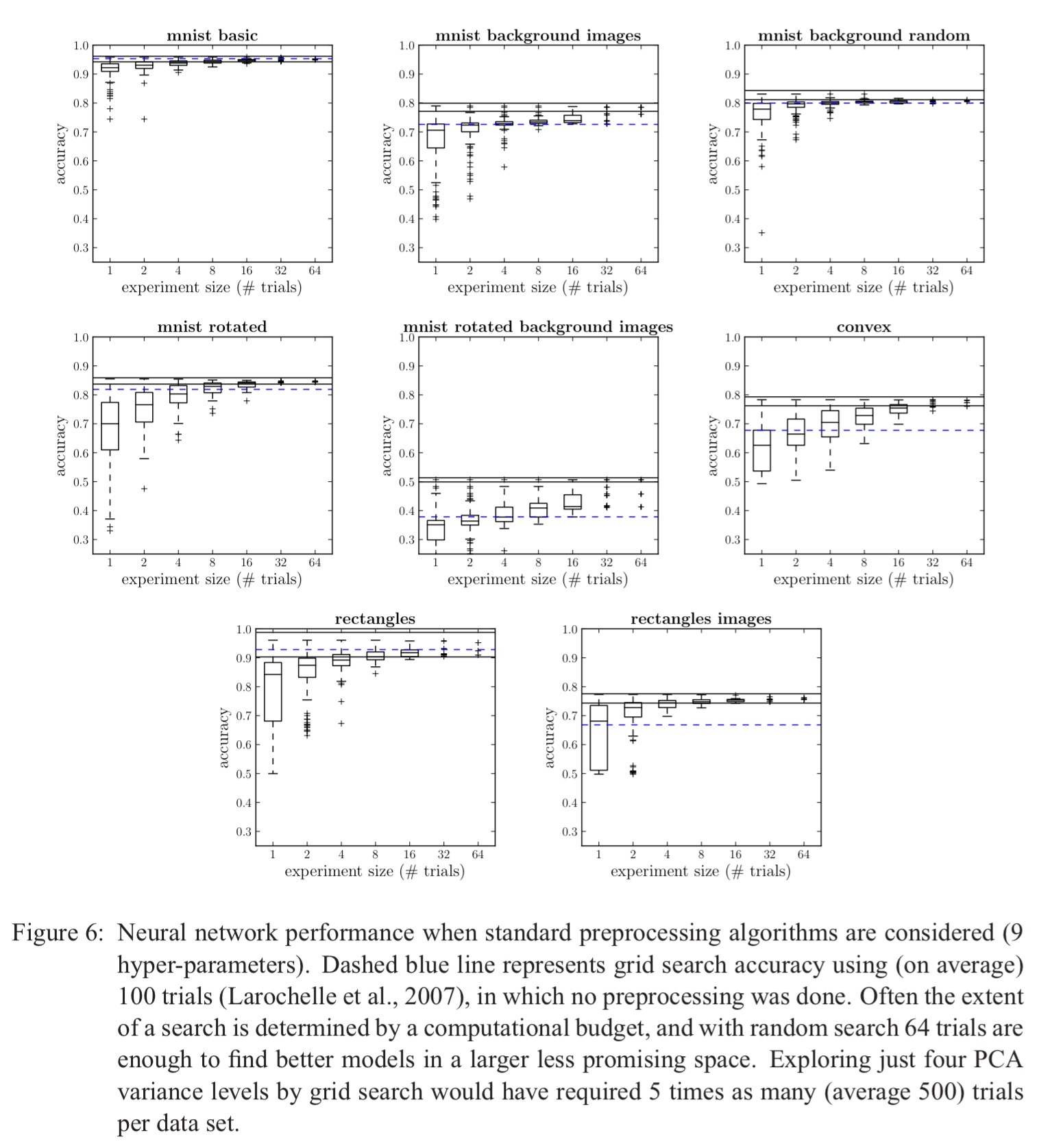
Now that we know how to interpret those curves, here are the results of neural network hyper-parameter optimisation experiments using random search, as compared to grid search (the blue line):
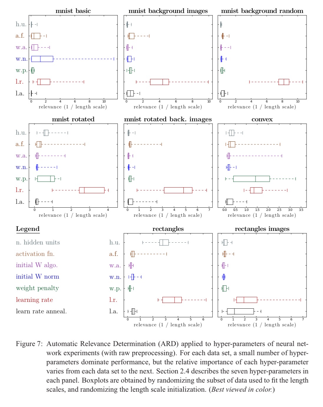
And this plot reinforces the point that only a small number of parameters are significant in each case, but the relative important of each individual hyper-parameter varies from one dataset to the next:
Deep networks have way more hyper-parameters, and we’d expect manual search to have more impact here. Experiments with a Deep Belief Network (DBN) with 32 hyper-parameters across 8 different datasets showed that random search found a better model than manual search for one dataset, an equally good model in four, and an inferior model in three.
In this more challenging optimization problem, random search is still effective, but not superior as it was in the case of neural network optimisation.
There is a huge body of work on global optimisation, much of which could be applied to hyper-parameter optimisation. However, grid search and random search have the advantage of being very simple to understand and implement.
With so many sophisticated algorithms to draw on, it may seem strange that grid search is still widely used, and, with straight faces, we now suggest using random search instead. We believe the reason for this state of affairs is a technical one. Manual optimization followed by grid search is easy to implement: grid search requires very little code infrastructure beyond access to a cluster of computers. Random search is just as simple to carry out, uses the same tools, and fits in the same workflow. Adaptive search algorithms on the other hand require more code complexity. They require client-server architectures in which a master process keeps track of the trials that have completed, the trials that are in progress, the trials that were started but failed to complete.
Improving neural networks by preventing co-adaptation of feature detectors
This short paper presents a very simple technique to reduce overfitting when training networks. For each training example presented to the network, each hidden unit is randomly omitted with probability 0.5. We call this dropout. Dropout prevents complex co-adaptations of feature detectors since a given hidden unit cannot rely on other hidden units being present. This ensures each neuron learns to make an independently useful contribution.
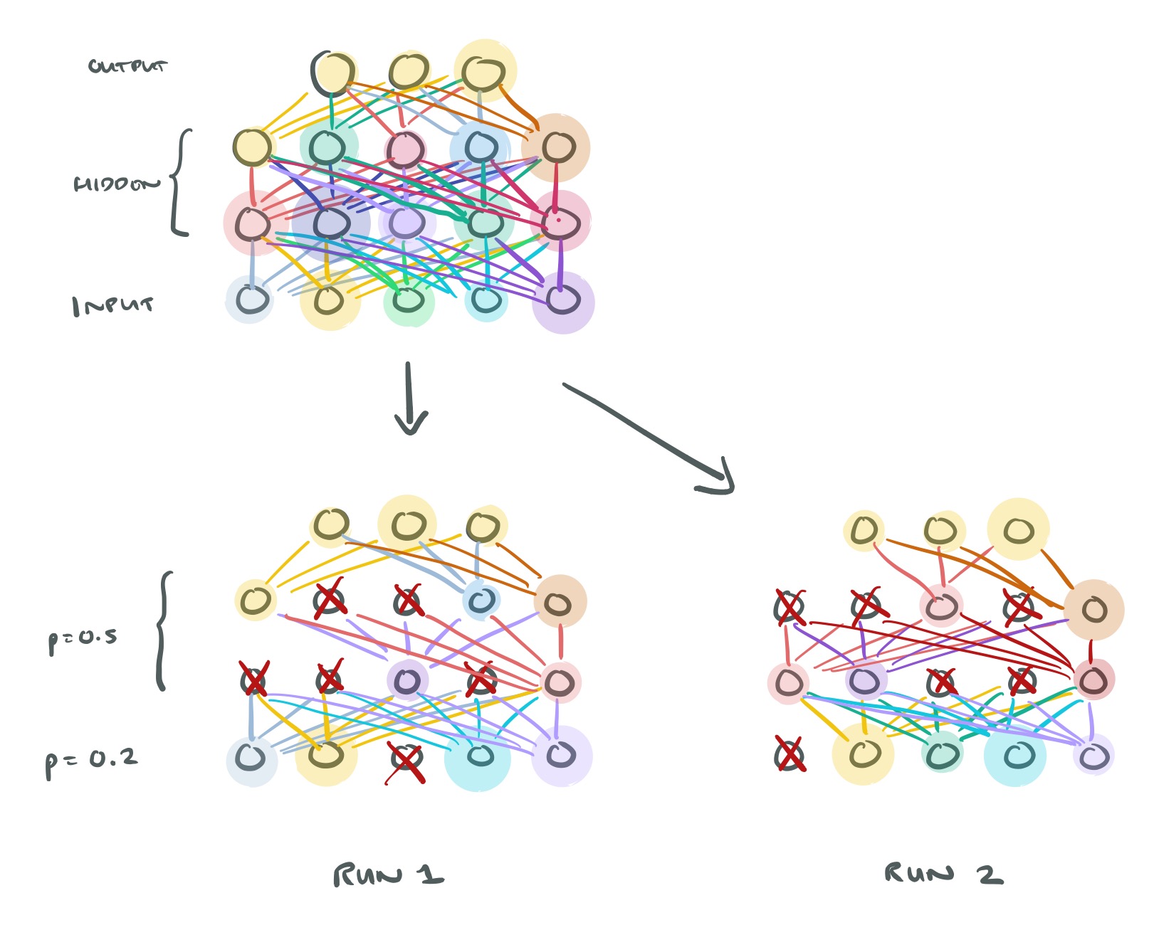
Another way to view the dropout procedure is as a very efficient way of performing model averaging with neural networks. A good way to reduce the error on the test set is to average the predictions produced by a very large number of different networks. The standard way to do this is to train many separate networks and then to apply each of these networks to the test data, but this is computationally expensive during both training and testing. Random dropout makes it possible to train a huge number of different networks in a reasonable time. There is almost certainly a different network for each presentation of each training case but all of these networks share the same weights for the hidden units that are present.
Here’s an example of dropout at work, where you can see it makes a big difference to the test error.
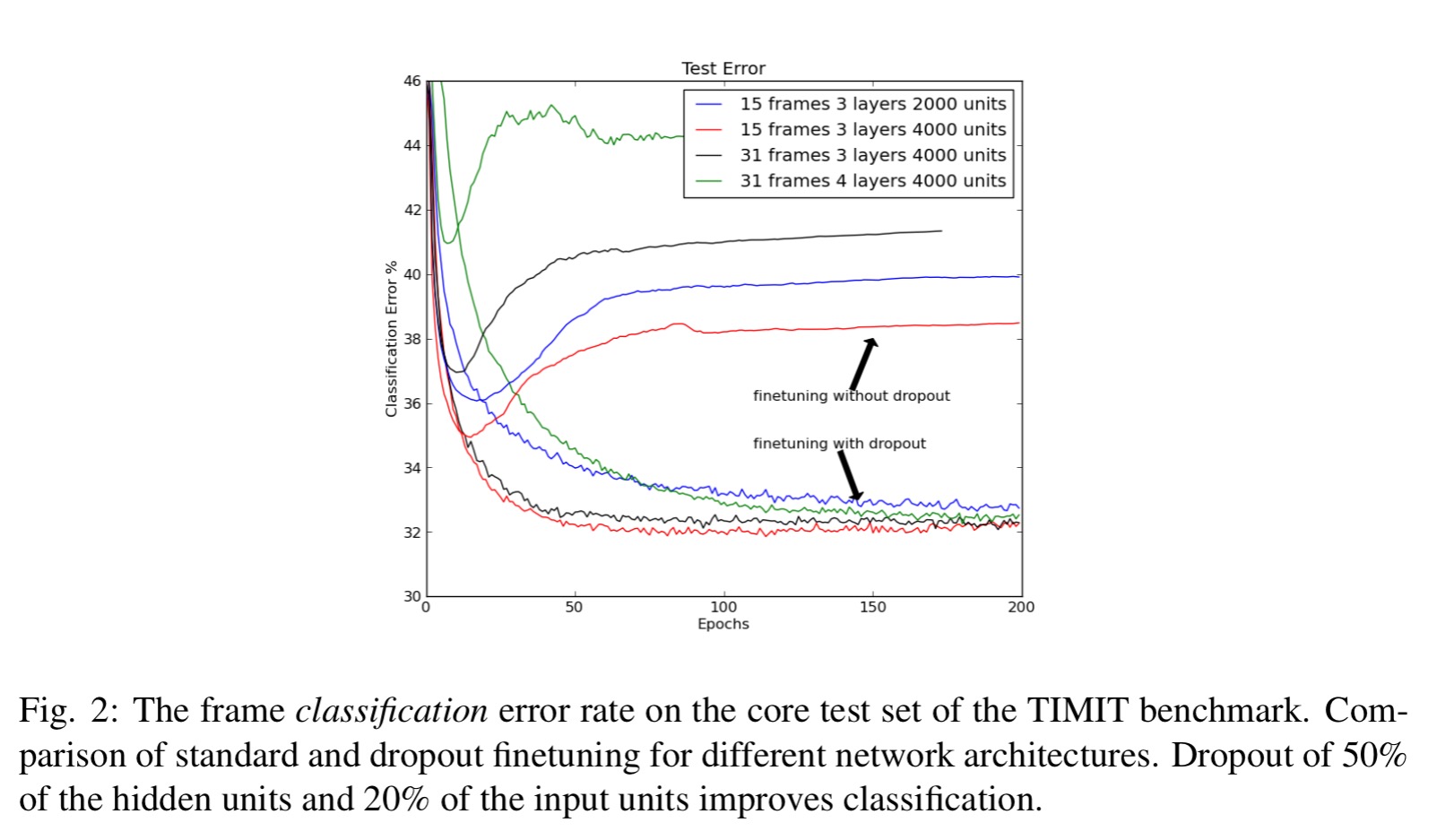
After some experimentation, a dropout probability of 50% for hidden layers and 20% for input units seems to work well.
Dropout: a simple way to prevent neural networks from overfitting
This is a longer paper from many of the same authors exploring the same fundamental idea as above. We get a much more comprehensive set of evaluations, which show that dropout can improve neural net performance in a wide variety of application domains including object classification, digit recognition, speech recognition, document classification, and analysis of computational biology data. “This suggests that dropout is a general technique and is not specific to any domain.” The idea can also be extended to other models, and the authors show an application with Restricted Boltzman Machines.
We also get a slightly deeper explanation of what’s going on when dropout is used, and how to test using a model trained using dropout:
Applying dropout to a neural network amounts to sampling a “thinned” network from it. The thinned network consists of all the units that survived dropout. A neural net with n units, can be seen as a collection of 2n possible thinned neural networks. These networks all share weights so that the total number of parameters is still O(n2), or less. For each presentation of each training case, a new thinned network is sampled and trained. So training a neural network with dropout can be seen as training a collection of 2n thinned networks with extensive weight sharing, where each thinned network gets trained very rarely, if at all.
At test time, you use the network as a single neural net, but with weights that are scaled-down versions of the trained weights. If a unit is retained with probability p during training, the outgoing weights of that unit are multiplied by p when testing.
A form of regularisation called max-norm regularisation was found to work well in conjunction with dropout. This simply constrains the norm of the weight vector at each hidden unit to be (upper) bounded by a fixed constant c (clipping). If w is the vector of weights, then we want .
Although dropout alone gives significant improvements, using dropout along with max-norm regularization, large decaying learning rates and high momentum provides a significant boost over just using dropout.
Dropout does have one disadvantage: it increases training by a factor of 2-3. Thus you can trade off between overfitting and training time by tweaking the dropout rate.
Appendix A contains some useful hints for training dropout networks in practice.
Adam: a method for stochastic optimization
Stochastic gradient-based optimization is of core practical importance in many fields of science and engineering… Stochastic gradient descent proved itself as an efficient and effective optimization method that was central in many machine learning success stories, such as recent advances in deep learning.
Adam is a stochastic optimisation technique for high-dimensional parameter spaces and noisy objectives (such as the noise introduced by using dropouts). It has per-parameter adaptive learning rates, and combines the advantages of two recent methods you may have seen popping up in papers: AdaGrad and RMSProp. It also works well in online settings, is straightforward to implement, and requires little memory.
Some of Adam’s advantages are that the magnitudes of parameter updates are invariant to rescaling of the gradient, its stepsizes are approximately bounded by the stepsize hyper-parameter, it does not require a stationary objective, it works well with sparse gradients, and it naturally performs a form of step size annealing.
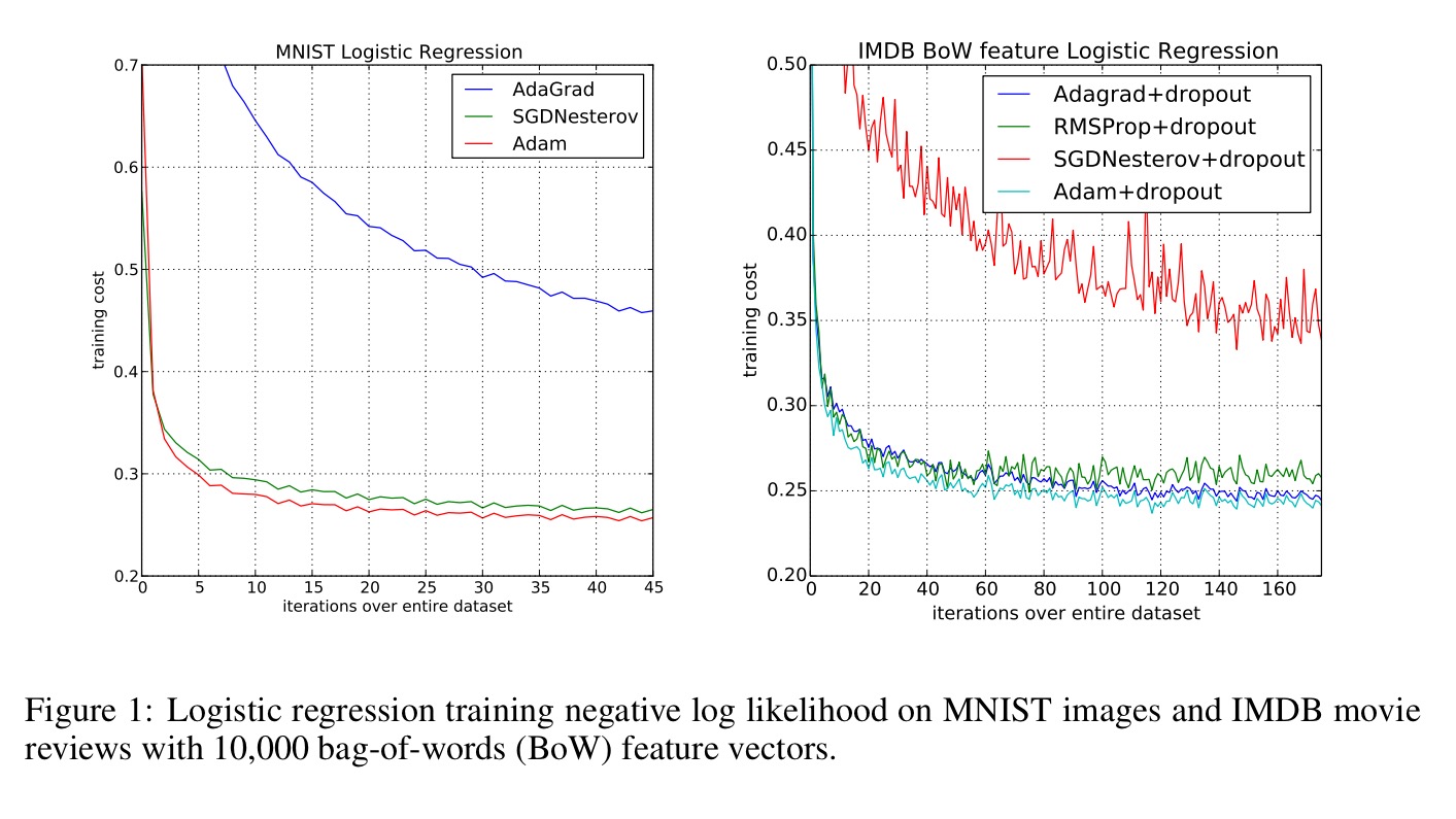
When used in logistic regression, Adam gives similar convergence as SGD with momentum (Nesterov), and faster convergence than Adagrad:
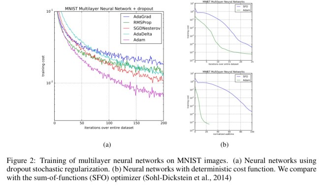
Fast convergence is also demonstrated with MNIST multi-layer neural networks :
And finally, Adam gives very impressive results when used with convolutional neural networks.
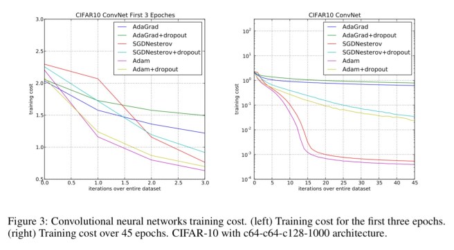
Overall, we found Adam to be robust and well-suited to a wide range of non-convex optimization problems in the field of machine learning.
The pseudo-code for Adam is shown below:
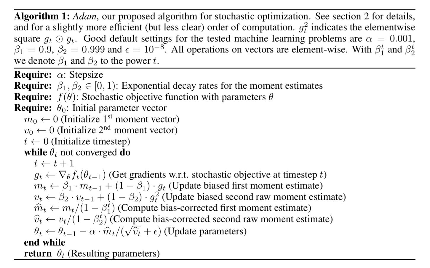
The algorithm updates exponential moving averages of the gradient (mt) and the squared gradient (vt) where the hyper-parameters β1, β2 ∈ [0, 1) control the exponential decay rates of these moving averages. The moving averages themselves are estimates of the 1st moment (the mean) and the 2nd raw moment (the uncentered variance) of the gradient. However, these moving averages are initialized as (vectors of) 0’s, leading to moment estimates that are biased towards zero, especially during the initial timesteps, and especially when the decay rates are small (i.e. the βs are close to 1). The good news is that this initialization bias can be easily counteracted, resulting in bias-corrected estimates
and
.
Initialization bias correction is discussed in section 3 of the paper, the short version is that you divide by to correct the first moment estimate, and by
to correct the second moment estimate (as can be seen in the algorithm pseudocode).
The hyper-parameter α sets an upper bound on the magnitude of steps in parameter space, and therefore “we can often deduce the right order of magnitude of α such that optima can be reached from θ0 within some number of iterations.”
Sebastian Ruder has a very helpful blog post entitled “An overview of gradient descent optimisation algorithms” that starts with vanilla SGD, shows some of the issues with it, and introduces a series of algorithms leading up to Adam that gradually chip away at those issues. There’s a nice animated visualisation too.
Batch normalization: accelerating deep network training by reducing internal covariate shift
Network training converges faster if inputs to the network are whitened. That is, inputs are linearly transformed to have zero means and unit variances. But consider a multi-layer network, by the time we’re a few layers in, the inputs to layer n are now some combinations of the outputs of layer n-1, and as training progresses we lose the normalisation effect. This brings back some of the problems than normalisation/whitening are intended to reduce: vanishing gradients, slow training, and saturation.
The fancy name for this change in the distributions of the internal nodes of a deep network over the course of time during training is Internal Covariate Shift. The central idea of batch normalisation is to bring back the benefits of normalisation not just for the initial inputs, but at every layer of the network. In theory this would give us faster convergence, and in practice it seems to be much faster:
… we apply Batch Normalization to the best-performing ImageNet classification network, and show that we can match its performance using only 7% of the training steps…
(I’ll just pause there for a moment to let that sink in)
… and can further exceed its accuracy by a substantial margin. Using an ensemble of such networks trained with Batch Normalization, we achieve a top-5 error rate that improves upon the best known results on ImageNet classification.
In batch normalisation, each scalar feature in a layer is independently normalised by making it have a mean of zero and variance of 1. For the kth dimension:
where the expectation and variance are computed over the training set data. Assuming mini-batch based stochastic gradient descent training, then in each mini-batch we will produce estimates of the mean and variance of each activation. “This way, the statistics used for normalization can fully participate in the gradient backpropagation.”
The full Batch Normalization Transform is as follows, where &eps; is a constant added to the mini-batch variance for numerical stability:
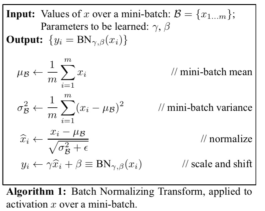
The parameters γ and β are used to scale and shift the normalized value, so that normalisation does not end up constraining what the layer can represent.
To Batch-Normalize a network, we specify a subset of activations and insert the BN transform for each of them, according to Alg. 1. Any layer that previously received x as the input, now receives BN(x). A model employing Batch Normalization can be trained using batch gradient descent, or Stochastic Gradient Descent with a mini-batch size m \> 1, or with any of its variants such as Adagrad [or Adam].
When using batch normalisation, the following changes are also recommended:
- increasing the learning rate (batch normalisation allows faster learning with no adverse effects)
- removing dropout (batch normalisation achieves some of the same goals, and avoids overfitting)
- reducing L2 weight regularization (by a factor of 5 in the author’s tests)
- accelerating the learning rate decay (6x faster)
- removing local response normalisation if you are using it
- shuffle training examples more thoroughly
- use less distortion of images in training sets, to let the trainer focus more on ‘real’ images
Delving deep into rectifiers: surpassing human-level performance on ImageNet classification
… the rectifier neuron, Rectified Linear Unit (ReLU) is one of several keys to the recent success of deep networks. It expedites convergence of the training procedure and leads to better solutions than conventional sigmoid-like units. Despite the prevalence of rectifier networks, recent improvements of models and theoretical guidelines for training them have rarely focused on the properties of the rectifiers.
In other words, everybody is just using the standard ReLU that looks like this:
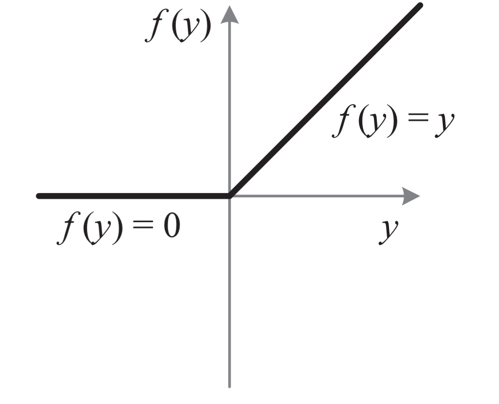
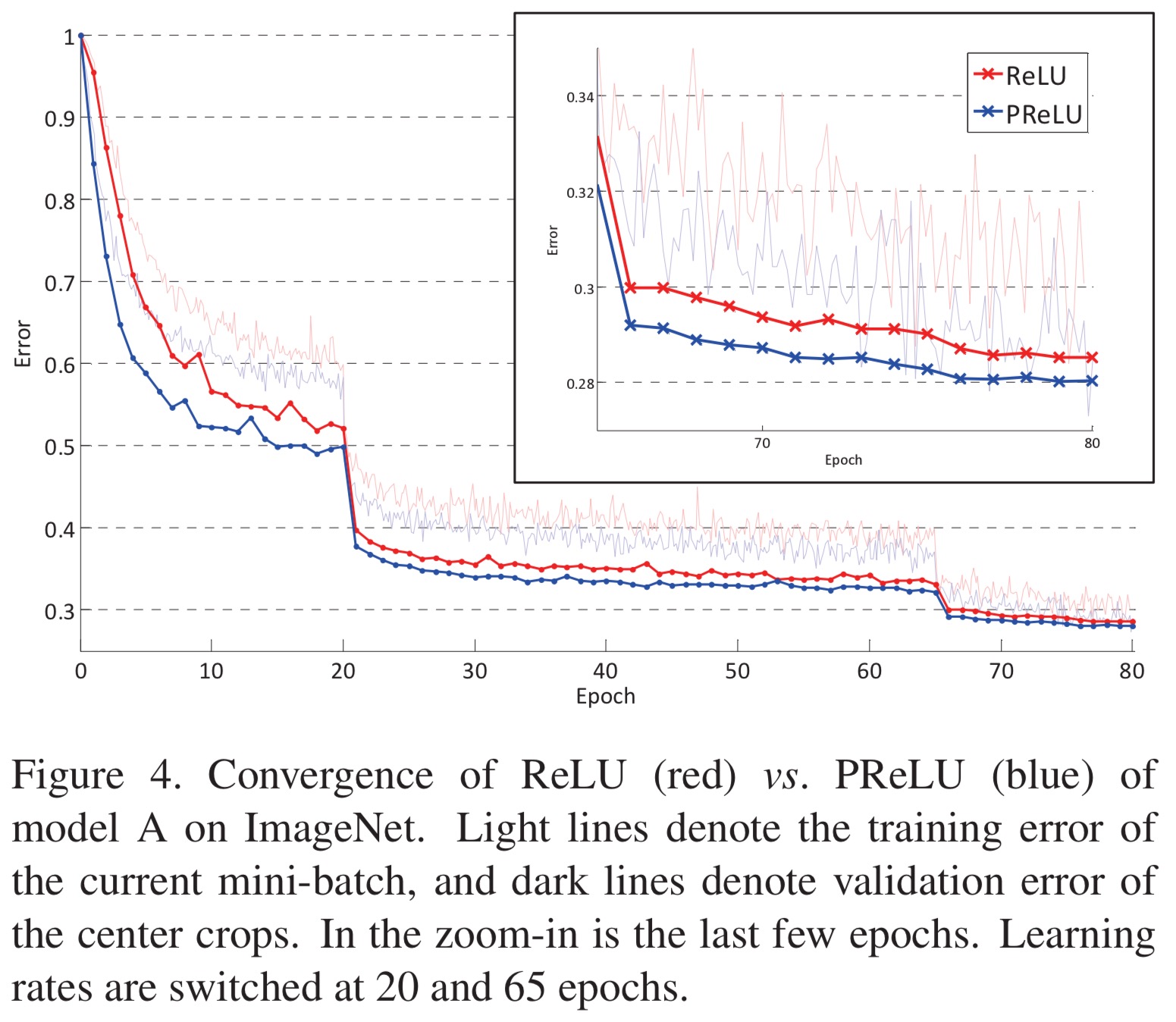
The authors make two key advances in this paper. Firstly they show a modified version of the standard ReLU, called a Parametric Rectified Linear Unit (PReLu) which can adaptively learn the parameters of the rectifiers, improving accuracy at negligible extra computing cost. Secondly they introduce a new method for initialising parameters which helps with the convergence of very deep models trained directly from scratch.
Do these enhancements make a big difference? Yes!
Based on the learnable activation and advanced initialization, we achieve 4.94% top-5 test error on the ImageNet 2012 classification dataset. This is a 26% relative improvement over the ILSVRC 2014 winner (GoogLeNet, 6.66%). To our knowledge, our result is the first to surpass the reported human-level performance (5.1%,) on this dataset.
PReLus have a learned parameter a which controls the slope of the negative part:
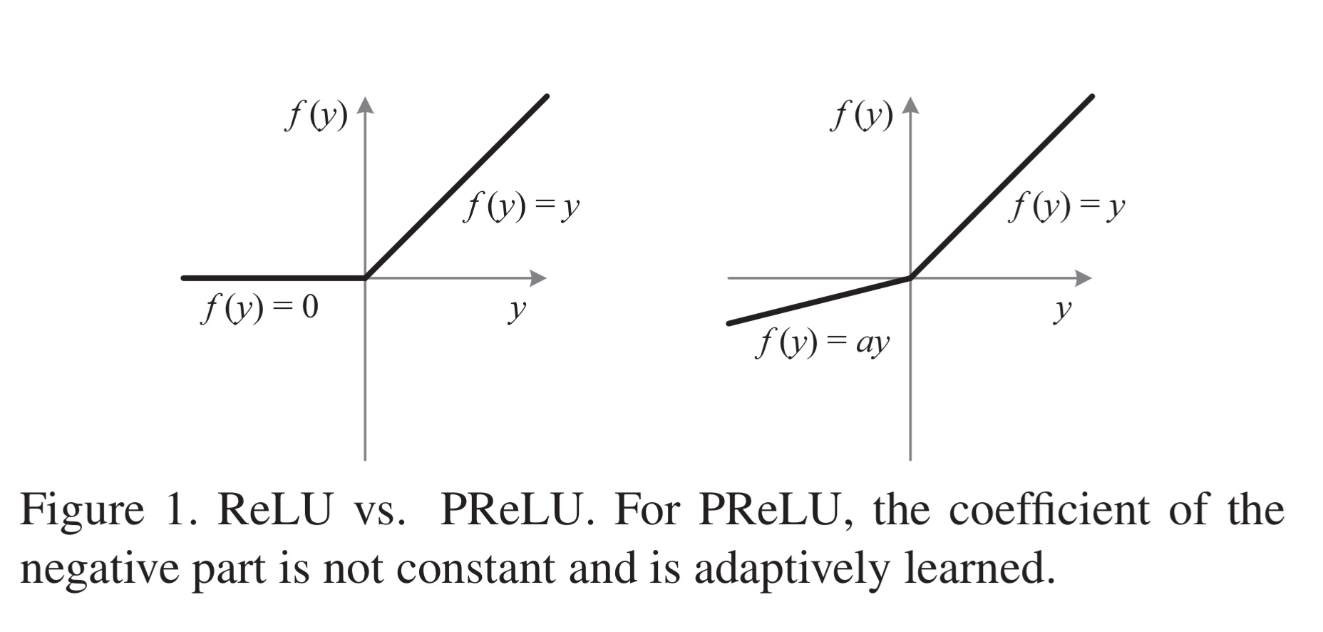
(Note that when a is small and fixed, PReLu becomes Leaky ReLU).
PreLU is trained using backpropagation and optimized simultaneously with other layers.
Rectifier networks are easier to train than tradititional sigmoid-like activation networks, but a bad initialization can still hamper the learning of a highly non-linear system…
Deep CNNs are typically initialised with random weights drawn from Gaussian distribution, but this can lead to situations where the magnitudes of input signals are reduced or magnified exponentially. Instead, it is better to draw initial weights from a zero-mean Gaussian distribution with standard deviation for forward propagation, and
for backpropagation (
is the number of connections in the layer). Doing this avoids the exponential problem. See §2.2 for the full gory details.
I think it might be of interest to describe our approach to hyper parameters optimization.
We have implemented an hybrid algorithm that combines ideas of simulated annealing, genetic search and grid search.
It uses a continually decreasing probability of choosing to explore (a) or adjust known good points (b).
a) exploring phase: it looks at largest unexplored regions and halve it. (Similar to grid search)
b) adjustment phase:
1. Data points are assigned a probability based it’s closest neighbors scores (distance weighted average score)
2. Weighted roulette to select a data point and mutate it in all directions with a gaussian process
After a fixed number of iterations or after a number of iterations without improvements, the point (set of parameters) with the highest evaluation value is returned.