REX: A development platform and online learning approach for runtime emergent software systems Porter et al. OSDI 2016
If you can get beyond the (for my taste, ymmv) somewhat grand claims and odd turns of phrase (e.g., “how the software ‘feels’ at a given point in time” => metrics) then there’s something quite interesting at the core of this paper. Given a system in which there are multiple different implementations of system components (interface implementations) – for example, each using differing algorithms with differing properties – how do you select the best-performing combination of components at any given point in time?
It almost sounds like a non-problem (who has lots of different implementations of each component of their system sitting around just in case…?), but the motivating web server example persuaded me not to dismiss it out of hand, and you can imagine the same approach being used for selecting amongst configuration options that have major impacts on runtime strategy as well.
The authors study a web server with two major internal component interfaces the RequestHandler interface, and the HTTPHandler interface. There are thread-per-client and thread-pool strategy implementations of the request handler interface, and four implementations of the http handler interface covering all combinations of caching/non-caching and compressing/non-compressing. Caching can be achieved using a number of different cache implementations, and likewise for compression:

All told in fact, the web server has over 30 different components (not all shown in the above figure), leading to 42 different possible ways of assembling a web server.
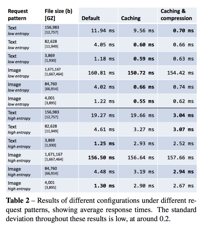
The evaluation shows that the component combinations which give the best performance at any point in time depend very much on the workload characteristics. For example, the type of resources most commonly requested (text or image), the size of the returned documents, and how diverse a set of documents are requested (‘entropy’ in the table below):

What the team set out to do is build a system that learns the best combinations under different conditions and adapts the runtime configuration accordingly as the workload changes.
These results confirm there are different optimal configurations of components that can form our target system in different environments. Low entropy and high text conditions favor configurations with caching and compression; low entropy and low text conditions favor configurations with caching only; and high entropy conditions favor a mixture of configurations. The subtleties within these results, and the fact that issues such as disk/memory latency will vary across machines, further motivate a real-time, machine-learning-based solution to building software.
If you thought integration testing was bad before, wait till you try to debug a system that deliberately explores all possible combinations of components at runtime!!!
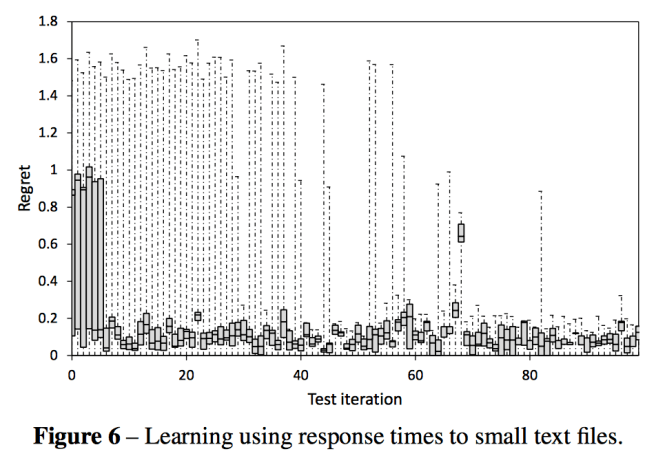
REX is the end result. Here it is learning the optimal configuration when given a workload of small text files. There is a big reduction in ‘regret’ after only a few iterations (each iteration lasting 10 seconds).

Regret is defined as ( 1/response_timechosen action – 1/response_timeoptimal action).
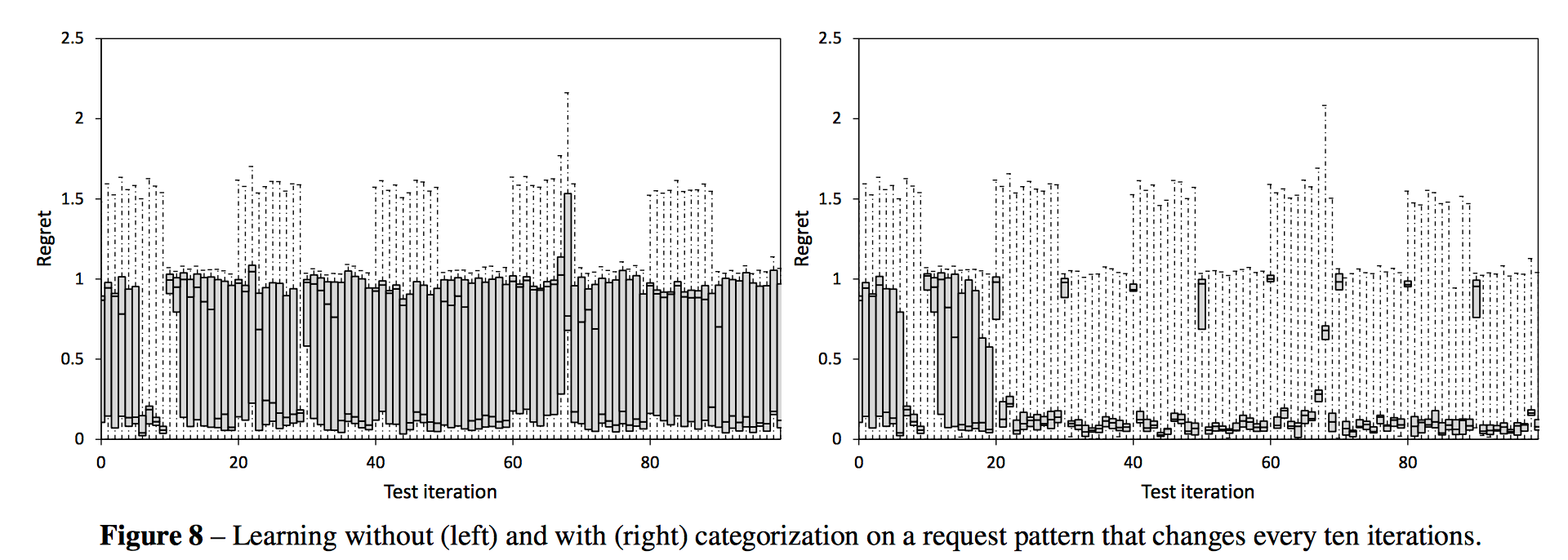
By including a categorization of workload as input to the learning algorithm, the system is able to adapt to changing workloads over time. This makes a big difference as shown below:
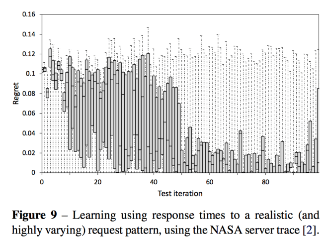
When you put it all together, you get a system that performs well with challenging real-world traces:
In Fig. 9 (below) we show results from a real-world web server workload of highly mixed resource requests, taken from the publicly available NASA server trace [2]. This is a challenging request pattern due to its high variance over time, in which different kinds of resource are requested in very different volumes. As a result our learning approach finds it more difficult to compare like-for-like results as different configurations are tested. Initially regret here is generally high, but decreases steadily up to the 40th iteration mark.

How it works
Building a system like REX requires a component programming model that facilitates runtime swapping of components. For that, the authors use their own component programming language called Dana. Dana proxies all objects flowing into and out of components and will keep mementos (‘transfer fields’) on behalf of component instances that can be used to hold state across different component implementations when the runtime decides to swap one implementation out for another one using a hot-swap mechanism.
When you start a Dana application, the first component is loaded and introspected to determine what components it needs (interfaces it depends on). Components implementing those interfaces are discovered in the project (this really isn’t new, sorry – see e.g., the way that Spring Boot does classpath scanning to discover components and configure itself at runtime). What is different though is that instead of selecting a single configuration, REX will build a list of all possible combinations, which will be systematically explored at runtime. To guide the exploration REX captures events arriving from the outside world, and metrics from the implementation. In the web server example the events are simply the arriving http requests and the sizes of the corresponding responses, and the chosen metric is the average response time. (No, mean latency is not generally a useful metric, but let’s roll with it for now…).
The interesting bit is how REX then learns the optimal configurations…
Online learning must balance the exploration of under-tested configurations with exploiting configurations already known to perform well. The canonical form of this is the multi-armed bandit problem, devised for clinical trials, and recently a dominant paradigm for optimization on the web. A multi-armed bandit has a set of available actions called arms. Each time an arm is chosen, a random reward is received, which depends (only) on the selected arm. The objective is to maximize the total reward obtained. While short-term reward is maximized by playing arms currently believed to have high reward, long-term benefit is maximized by exploring to ensure that we don’t fail to find the best arm.
Each ‘arm’ is a system configuration, and the reward given by ‘playing an arm’ (deploying a configuration) is determined by the metrics. Thompson sampling is used for the multi-armed bandit problem, in which each arm is played proportionally to the probability that it is the best arm given the information to date. Bayesian inference is used to produce ‘posterior distributions’ encoding beliefs about the expected values of configurations, which are modeled as bell curves.
The center of the bell curve represents the average reward seen on that arm to date, and the spread of the curve represents the level of uncertainty. When a Thompson sample is taken from such a curve, for the corresponding arm to be played it must either have a high average (representing the case where we know a configuration to be good) or a wide spread giving us the chance of drawing a high value (representing the case where we still have high uncertainty).
The effect is that the arms most likely to be played are those that experience suggests are likely to perform well, and those that may perform well but we have insufficient information about. Arms for which we have good information that they will perform badly are played with very low probability. As more information is gained, and beliefs concentrate on the truth, no arms will remain for which there is insufficient information. Thus, in the long term, optimal arms are played with very high probability.
Forming beliefs about all possible combinations of components could quickly give rise to very large numbers of combinations to explore.
We therefore follow and use a regression framework based on classical experimental design to share information across the different arms available to us… This is formalized by modelling the expected reward for a given configuration as a function of the components deployed within that configuration. In detail, we code each interface as a factor [categorical] variable, with number of levels equal to the number of available components for that interface.
Each possible component has a corresponding coefficient in the expected reward equation. Make an m x k ‘action’ matrix where each row m represents a configuration, and each column k represents a regression coefficient. After sampling a vector of coefficients Β, the matrix can be multiplied by this vector simultaneously solving for all configurations. The row with the highest resulting value is chosen and deployed. After ten seconds the resulting reward is observed (that doesn’t seem very long for e.g. caches to get warm???) and the result is stored. The posterior distribution is then updated before repeating the process.
To help the system ‘unlearn’ what it already knows when the workload characteristics change, additional features are added which represent the current workload. In the current system, these features were manually defined by the authors as the workload entropy (# of different resources requested in a given time frame) and text volume (% of content requested in a given timeframe that was textual). Terms are added to the expected reward equation capturing these variables.
A final thought : it would be interesting to compare the results to the behaviour of a DQN trained to explore the same state space and maximise its reward… Actions taken by the agent would simply correspond to deploying a given configuration, and the Q reward function would be determined by the resulting runtime metrics.
