ImageNet Classification with Deep Convolutional Neural Networks – Krizhevsky et al. 2012

Like the large-vocabulary speech recognition paper we looked at yesterday, today’s paper has also been described as a landmark paper in the history of deep learning. It’s also a surprisingly easy read!

The ImageNet dataset contains over 15 million labeled high-resolution images of objects in roughly 22,000 categories. The annual ImageNet Large-Scale Visual Recognition Challenge (ILSVRC) competition uses a subset of ImageNet with roughly 1000 images in each of 1000 categories. There are 1.2M training images, 50,000 validation images, and 150,000 testing images. For reporting error rates, a model predicts the top 5 most likely labels. The ‘top-5’ error rate is the fraction of test images for which the correct label is amongst this top 5, and the ‘top-1’ error rate is the fraction of test images for which the correct label is the one judged most likely by the model.

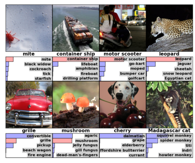
Using an eight-layer neural network with five convolutional layers, the authors achieved top-1 and top-5 error rates on the ILSVRC-2010 dataset of 37.5% and 17.0% – considerably better than the previous state-of-the-art at 45.7% and 25.7% respectively. The model was trained using two GPUs.

(In the 2014 ILSVRC competition a 19-layer CNN achieved a 7.5% top-5 error rate. In the 2015 competition, an ensemble containing 152-layer networks achieved a 3.57% top-5 error rate!).

Our results show that a large, deep convolutional neural network is capable of achieving record-breaking results on a highly challenging dataset using purely supervised learning. It is notable that our network’s performance degrades if a single convolutional layer is removed. For example, removing any of the middle layers results in a loss of about 2% for the top-1 performance of the network. So the depth really is important for achieving our results. To simplify our experiments, we did not use any unsupervised pre-training even though we expect that it will help, especially if we obtain enough computational power to significantly increase the size of the network without obtaining a corresponding increase in the amount of labeled data.

Data Augmentation

In order to avoid overfitting we’d ideally like a larger dataset. Since the ImageNet dataset size is fixed, we can artificially enlarge it using ‘label-preserving transformations.’ Take one of the original 256×256 input images, and extract random 224×224 patches from it (as well as their horizontal reflections). We can then train on these extracted patches:

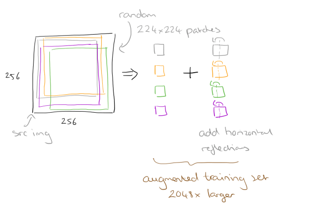
A second form of augmentation is to alter the intensities in the RGB channels in the training images. A Principle Component Analysis is performed, and multiples of the found principle components can be added. “This scheme approximately captures an important property of natural images, namely, that object identity is invariant to changes in the intensity and color of the illumination.”

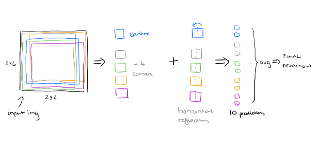
At test time, the network makes a prediction by extracting five 224×224 patches (the four corner patches and the center patch) as well as their horizontal reflections (hence ten patches in all), and averaging the predictions made by the network’s softmax layer on the ten patches.

Network Structure

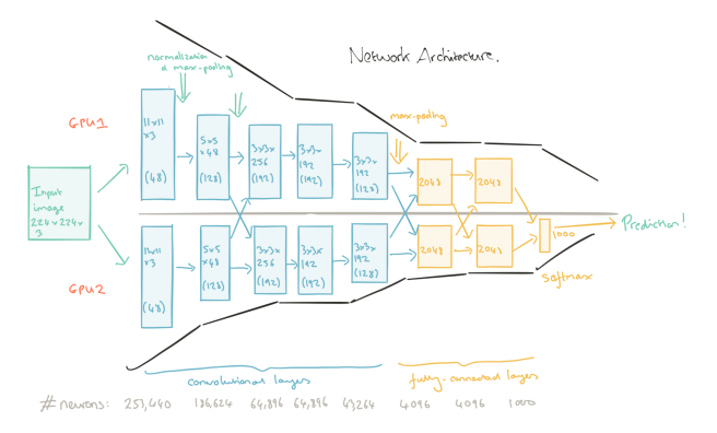
Let’s take a look at the structure of the network, and how data flows from input images to final classification prediction.

(click on the image for a larger view).

Network training is split across two GPUs. “The parallelization scheme we employ essentially puts half of the kernels (or neurons) on each GPU, with one additional trick: the GPUs communicate only in certain layers. This means that, for example, the kernels of layer 3 take input from all kernal maps in layer 2. However, kernels in layer 4 take input only from those kernel maps in layer 3 which reside on the same GPU…”

The first five layers of the network are convolutional, and the last three are fully connected. The output of the last layer is fed to a 1000-way softmax which produces a distribution over the 1000 class labels.

The first convolutional layer filters the 224×224×3 input image with 96 kernels of size 11×11×3 with a stride of 4 pixels. The second convolutional layer takes as input the (response-normalized and pooled) output of the first convolutional layer and filters it with 256 kernels of size 5 × 5 × 48The third, fourth, and fifth convolutional layers are connected to one another without any intervening pooling or normalization layers. The third convolutional layer has 384 kernels of size 3 × 3 ×256 connected to the (normalized, pooled) outputs of the second convolutional layer. The fourth convolutional layer has 384 kernels of size 3 × 3 × 192 , and the fifth convolutional layer has 256 kernels of size 3 × 3 × 192. The fully-connected layers have 4096 neurons each.

The following figure shows the 11x11x3 convolutional kernels learned by the first convolutional layer.

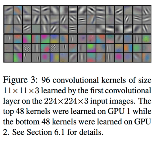
The top 48 kernels were learned on GPU 1, while the bottom 48 kernels were learned on GPU 2… The kernels on GPU 1 are largely color-agnostic, while the kernels on GPU 2 are largely color specific. This kind of specialization occurs during every run and is independent of any particular random weight initialization.

For the pooling layers, it is traditional to use non-overlapping neighbourhoods.

To be more precise, a pooling layer can be thought of as consisting of a grid of pooling units spaced s pixels apart, each summarizing a neighborhood of size z x z centered at the location of the pooling unit. If we set s=z we obtain traditional local pooling as commonly employed in CNNs. If we set s < z we obtain overlapping pooling. The authors use s = 2, z = 3 and found that this reduces the top-1 and top-5 error rates by 0.4% and 0.3% respectively compared to the non-overlapping s = z = 2 scheme. “We generally observe during training that models with overlapping pooling find it slightly more difficult to overfit.” Another technique used to combat overfitting is dropout. It simulates the effect of combining the predictions of many different models: > The recently introduced technique, called “dropout,” consists of setting to zero the output of each hidden neuron with probability 0.5. The neurons which are “dropped out” in this way do not contributed to the forward pass and do not participate in backpropagation. So every time an input is presented, the neural network samples a different architecture, but all these architectures share weights.

At testing time, all neurons are used with their outputs multiplied by 0.5. This approximates the geometric mean of the predictive distributions produced by the exponentially-many dropout networks.

We use dropout in the first two fully-connected layers… Without dropout, our network exhibits substantial overfitting. Dropout roughly doubles the number of iterations required to converge.

Efficiency

The standard way to model a neuron’s output f as a function of its input x is with f(x) = tanh(x) or f(x) = (1+e^-x)^-1. In terms of training time with gradient descent, these saturating nonlinearities are much slower than the non-saturating nonlinearity f(x) = max(0,x).

Neurons using f(x) = max(0,x) are called Rectified Linear Units (ReLUs). Networks with ReLUs train much faster than their equivalents with tanh units. “We would not have been able to experiment with such large neural networks for this work if we had used traditional saturating neuron models.”

ReLUs do not require input normalization to prevent them from saturating, but the authors found that a local normalization scheme aided generalization. Response normalization reduces the top-1 and top-5 error rates by 1.4% and 1.2% respectively.

(Wei Di has a nice visual comparison of activation functions on her blog):

Learned Knowledge

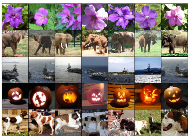
…Another way to probe the network’s visual knowledge is to consider the feature activations induced by an image at the last, 4096-dimensional hidden layer. If two images produce feature activation vectors with a small Euclidean separation, we can say that the higher levels of the neural network consider them to be similar. Figure 4 shows five images from the test set and the six images from the training set that are most similar to each of them according to this measure. Notice that at the pixel level, the retrieved training images are generally not close in L2 to the query images in the first column. For example, the retrieved dogs and elephants appear in a variety of poses. We present the results for many more test images in the supplementary material.