Distributed TensorFlow with MPI – Vishnu et al. 2016
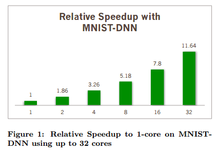
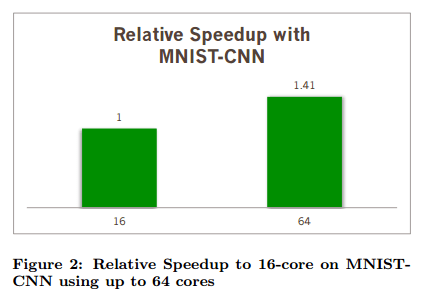
A short early release paper to close out the week this week, which looks at how to support machine learning and data mining (MLDM) with Google’s TensorFlow in a distributed setting. The paper also contains some good background on TensorFlow itself as well as MPI – and why MPI was preferred over Hadoop and Spark for this work. The results show performance improvements, but not in proportion to the amount of extra compute thrown at the problem (from 1 core to 32 cores on MNIST-DNN is a 11.64x improvement, and from 16 cores to 64 cores on MNIST-CNN is a 1.41x improvement for example).
TensorFlow
Deep Learning algorithms use multiple layers of neurons interconnected with synapses, and learn the weights for the synapses using gradient descent methods. Within Deep Learning, there are DNNs, CNNs, and RNNs.
- Deep Neural Networks (DNNs) are typically used on tabular datasets
- Convolutional Neural Networks (CNNs) are typically used on images
- Recurrent Neural Networks (RNNs) are typically used on time-dependent datasets.
Google’s TensorFlow readily supports DNNs, CNNs, and RNNs on multi-core and many-core (GPU) systems. Out of the box, TensorFlow is however restricted to single node usage.
The basic unit in TensorFlow is the computational graph. This graph contains nodes, which are operations, and edges which represent tensors (arbitrary dimensional arrays). Each node can take multiple inputs and give multiple outputs, with tensors created and passed from one node to another and, generically, deleted after use to avoid memory clutter. In addition to carrying tensors, edges can also be used to control the flow of a computation. Control dependencies can be used to enforce relationships such that some computations must be done before others, no matter what parallelization has occurred.
Placeholder tensors are where input enters a graph. Variables are tensors that are stored by the computational graph rather than being deleted after use. Variables can be used to store the weights of a model for example.
TensorFlow determines what order to compute the graph in by creating a queue of nodes with no dependencies. It keeps track of the number of unresolved dependencies for each node, and whenever it drops to zero, that node is put into the queue. The program then executes the nodes in the queue in some order, continuing to decrease the unresolved dependencies until it has computed the whole graph.
Each node in the graph is assigned to a device form computation (rather than running the whole graph in parallel on multiple devices). Assignment is greedy. Nodes are assiged to devices based on whether or not there is a kernel for that operation on that device (not all operations have GPU implementations for example), and based on which device is expected to be free when the computation is ready to be done.
Finally, TensorFlow inserts send and receive nodes between devices to transfer the tensors. It does this in a way to minimize communication (given the assignment of the graph) and modifies the graph assignments slightly if it changes the total execution time to change where communication happens.
Distributed TensorFlow
The three key design decisions in distributing TensorFlow were the choice of distributed programming model, the means of parallelizing the TensorFlow computation graph, and whether to use a synchronous or asynchronous update mechanism. The authors chose (a) MPI, (b) model parallelism, and (c) synchronous updates, respectively. A further pragmatic consideration was to make minimal changes to the TensorFlow codebase itself.
MPI
There are several programming models which may be used as a distributed memory implementation of TensorFlow. Specifically we considered several Mapreduce implementations including Hadoop and Spark. Hadoop was removed from consideration due to its frequent communication to the I/O subsystem. Spark – which considerably improves upon Hadoop by in-memory execution – was considered for distributed memory implementation. However, the current implementation of Spark runtime suffers from two primary issues: inability to take advantage of high performance communication networks using native interfaces (such as Verbs on InfiniBand, and PAMI on Blue Gene/Q networks); frequent I/O due to saving the key-value pairs for fault tolerance reasons. We addressed the limitations of Spark by using MPI as the communication interface…
MPI has its roots in supercomputing and is desgined to exploit the native communication interface as much as possible. When a native communication interface is not available and MPI falls back to using the sockets interface it becomes more equivalent to Spark. The authors’ implementation using the MPI All-to-all reduction primitive which allows operations such as sum on user data and disseminates the final results among all processes in a group.
We also observed that MPI has been criticized for its lack of support for fault tolerance. However, with recent advancements – such as User-level Fault Mitigation (ULFM) – and open source implementations, it is possible to design fault tolerant MLDM algorithms using MPI, without losing performance and ”continued execution” in the presence of hardware faults. We expect that with ULFM (or its variants) becoming available with mainstream implementations, MPI would find its wide acceptance in the MLDM community.
Model Parallelism
The initial process reads the samples from disk and splits them across processes. In the current implemenation, each device is considered of equal compute capacity. “We intend to address this limitation in the upcoming releases of our code.” The model is replicated on each device.
Each device learns the model independently using the standard backpropagation algorithm. This approach scales well in computation and communication, even though the model is replicated on each device… By using MPI and high performance communications, the overall fraction of time spent during computation is increased.
Sync or Async?
An important design choice is the synchronization of weights and biases with model parallelism. Several researchers have considered asynchronous methods for updating these data structures. While there are certain advantages of asynchronous updates – it becomes difficult to reason about the correctness of the algorithm and its equivalence to the standard gradient descent algorithms. Hence, we consider synchronous methods for updating the weights and biases.
The choice of MPI means communication overheads are lower, and the authors can take advantage of the heavily optimized averaging operation in MPI for synchronizing the data structures. “There are several well-known algorithms which implement the All-to-all reduction operation in log(p) time. Other interconnects such as Blue Gene and InfiniBand support these operations in hardware – further reducing the overall time complexity of the proposed implementation.”
Using synchronous communication is a big decision – I can certainly see it makes it easier to fit in with the existing TensorFlow algorithms with as little disturbance as possible. On the other hand, the barriers limit the overall speed-ups that can be achieved. Previously on The Morning Paper we looked at Petuum and Asychronous Compex Analytics in a Distributed Dataflow Architecture and in both cases the authors found considerable speed-ups from relaxing synchronization requirements.
Results
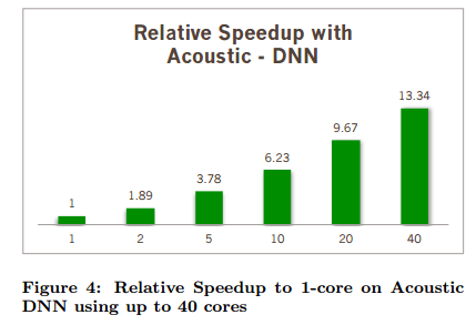
The distributed versions of TensorFlow do improve performance, but only to a limited degree compared to the increase in compute power being thrown at the problem. The evaluation section contains a number of graphs illustrating this (pay attention to the labels on the x-axis, uniform spacing does not equal uniform steps!). Here are a couple of examples:


It seems that the authors misuse the term “model parallelism”, while actually what they meant is “data parallelism”
It seems the authors misused the term “model parallelism” to mean “data parallelism”.