Simultaneous Localization and Mapping: Part I History of the SLAM problem – Durrant-Whyte & Bailey 2006

You can’t read far in robotics without encountering the SLAM problem. But what is it exactly? And what are the main approaches to solving it? Today’s paper provides an overview of the SLAM problem, a short history of research in the area, and an overview of the two main methods for solving it.

SLAM stands for Simultaneous Localization and Mapping. The challenge is to place a mobile robot at an unknown location in an unknown environment, and have the robot incrementally build a map of the environment and determine its own location within that map. Solving the SLAM problem provides a means to make a robot autonomous. For some outdoor applications, the need for location estimation is eliminated due the availability of high precision differential GPS sensors.

SLAM is a process by which a mobile robot can build a map of an environment and at the same time use this map to deduce its location. In SLAM, both the trajectory of the platform and the location of all landmarks are estimated online without the need for any a priori knowledge of location.

Figure 1 from the paper, reproduced below, shows a mobile robot moving through an environment, taking relative observations of unknown landmarks using a sensor located on the robot.

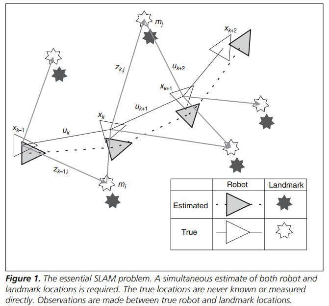
We can use this simple model to start to build up an understanding of the problem dimensions. At some instance of time k, the following quantities are defined:

• x_k, the state vector describing the location and orientation of the robot (i.e., where we think it is and which way we think it is facing)
• u_k, the control vector which was applied at time k-1 to drive the robot to a state x_k at time k.
• m_i, a vector describing the location of the ith landmark. Landmarks are assumed to be stationary (i.e. they don’t move over time).
• z_ik, an observation of the ith landmark taken from the robot at time k. Abbreviated to just z_k if the specific landmark is not relevant to the discussion.

We also build up knowledge of the set m of all landmarks, as well as X, U and Z the history of all robot locations, control inputs, and observations respectively.

Now we can express the SLAM problem in probabilistic terms. Given the history of all landmark observations and the history of the control inputs to some time k, and the initial location estimate x₀ we want to know the probability distribution for the current location of the robot and the landmarks. We can write this as:

P(x_k, m | Z_0:k, U_0,k, x₀)

Suppose we have an estimate for x and m at time k-1: P(x_k-1, m | Z_0:k-1, U_0,k-1). Now we follow a control input u_k and make an observation z_k. Given this, if we understand the effect of the control input and the observation, we can compute the posterior (estimates of locations at time k) using Bayes theorem.

This computation requires that a state transition model and an observation model are defined describing the effect of the control input and observation respectively.

The observation model tells us the probability of making an observation z_k when the locations of the robot and landmarks are known: P(z_k | x_k, m). The motion model is described in terms of a probability distribution on state transitions – more simply, the location at time k depends on where we were at time k-1, and the applied control input (note that it does not depend on any of the observations or the map): P(x_k | x_k-1, u_k).

If you’ve followed along so far, then we can plug the observation model and the motion model into “a standard two-step recursive (sequential) prediction (time-update) correction (measurement-update) form” :

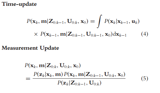
This part I just have to take on faith:).

The most important insight in SLAM was to realize that the correlations between landmark estimates increase monotonically as more and more observations are made. (These results have only been proved for the linear Gaussian case. Formal proof for the more general probabilistic case remains an open problem.) Practically, this means that knowledge of the relative location of landmarks always improves and never diverges, regardless of robot motion. In probabilistic terms, this means that the joint probability density on all landmarks P(m) becomes monotonically more peaked as more observations are made.

To see why each observation increases knowledge of the relative location of landmarks consider a simplified scenario with just two landmarks m₁ and m₂. The robot observes these from location x_k. Since landmarks don’t move (this is a condition of the problem defintion), the relative locations of m₁ and m₂ to each other are fixed for all time. The robot has an estimate of these relative locations from its observation at x_k. Now the robot moves to x_k+1 and is able to again observe m₂. This enables the estimates of the robots location x_k+1 and the location of m₂ to be updated. It also enables this to propagate back to update the location of m₁, even though m₁ was not seen from the new location, since the relative locations of m₁ and m₂ was known from previous measurements…

Turning all of this theory into executable algorithms requires finding an appropriate representation for the observation model and motion model that allows efficient and consistent computation of the prior and posterior distributions in the two-step recursive prediction form equations given above.

By far, the most common representation is in the form of a state-space model with additive Gaussian noise, leading to the use of the extended Kalman filter (EKF) to solve the SLAM problem. One important alternative representation is to describe the vehicle motion model as a set of samples of a more general non-Gaussian probability distribution. This leads to the use of the Rao-Blackwellized particle filter, or FastSLAM algorithm, to solve the SLAM problem. While EKF-SLAM and FastSLAM are the two most important solution methods, newer alternatives, which offer much potential, have been proposed, including the use of the information-state form.

An overview of both of these approaches is given in the paper – reproducing the necessary mathematics here would add little value over simply referring you directly to the appropriate sections on pages 103-106. For EKF-SLAM the motion model is based on a function of vehicle kinematics with added Guassion motion disturbances (fancy way of saying there’s a function than determines how the vehicle will move given its control inputs, with some noise added to account for real word discrepancies). The observation model is based on the ‘geometry of the observation’ (what you think you saw), also with some added noise. This allows you to use the standard statistical EKF method to compute mean and covariance of the posterior distribution. FastSLAM uses particle filtering (the ‘Rao-Blackwell’ bit is a way of reducing the sample space to make it tractable) with each particle defining a different vehicle trajectory hypothesis.

The wikipedia page on SLAM is also worth perusing, and if you want to run your own experiments, you can now get started with everything you need using Google’s Project Tango tablet development kit for Android.