BBR: Congestion-based congestion control Cardwell et al., ACM Queue Sep-Oct 2016
With thanks to Hossein Ghodse (@hossg) for recommending today’s paper selection.
This is the story of how members of Google’s make-tcp-fast project developed and deployed a new congestion control algorithm for TCP called BBR (for Bandwidth Bottleneck and Round-trip propagation time), leading to 2-25x throughput improvement over the previous loss-based congestion control CUBIC algorithm. In fact, the improvements would have been even more significant but for the fact that throughput became limited by the deployed TCP receive buffer size. Increasing this buffer size led to a huge 133x relative improvement with BBR (2Gbps), while CUBIC remained at 15Mbps. BBR is also being deployed on YouTube servers, with a small percentage of users being assigned BBR playback.
Playbacks using BBBR show significant improvement in all of YouTube’s quality-of-experience metrics, possibly because BBR’s behavior is more consistent and predictable… BBR reduces median RTT by 53 percent on average globally, and by more than 80 percent in the developing world.
TCP congestion and bottlenecks
The Internet isn’t working as well as it should, and many of the problems relate to TCP’s loss-based congestion control, even with the current best-of-breed CUBIC algorithm. This ties back to design decisions taken in the 1980’s when packet loss and congestion were synonymous due to technology limitations. That correspondence no longer holds so directly.
When bottleneck buffers are large, loss-based congestion control keeps them full, causing bufferbloat. When bottleneck buffers are small, loss-based congestion control misinterprets loss as a signal of congestion, leading to low throughput. Fixing these problems requires finding an alternative to loss-based congestion control.
From the perspective of TCP, the performance of an arbitrarily complex path is bound by two constraints: round-trip propagation time (RTprop), and bottleneck bandwidth, BtlBw (the bandwidth at the slowest link in each direction).
Here’s a picture to help make this clearer:
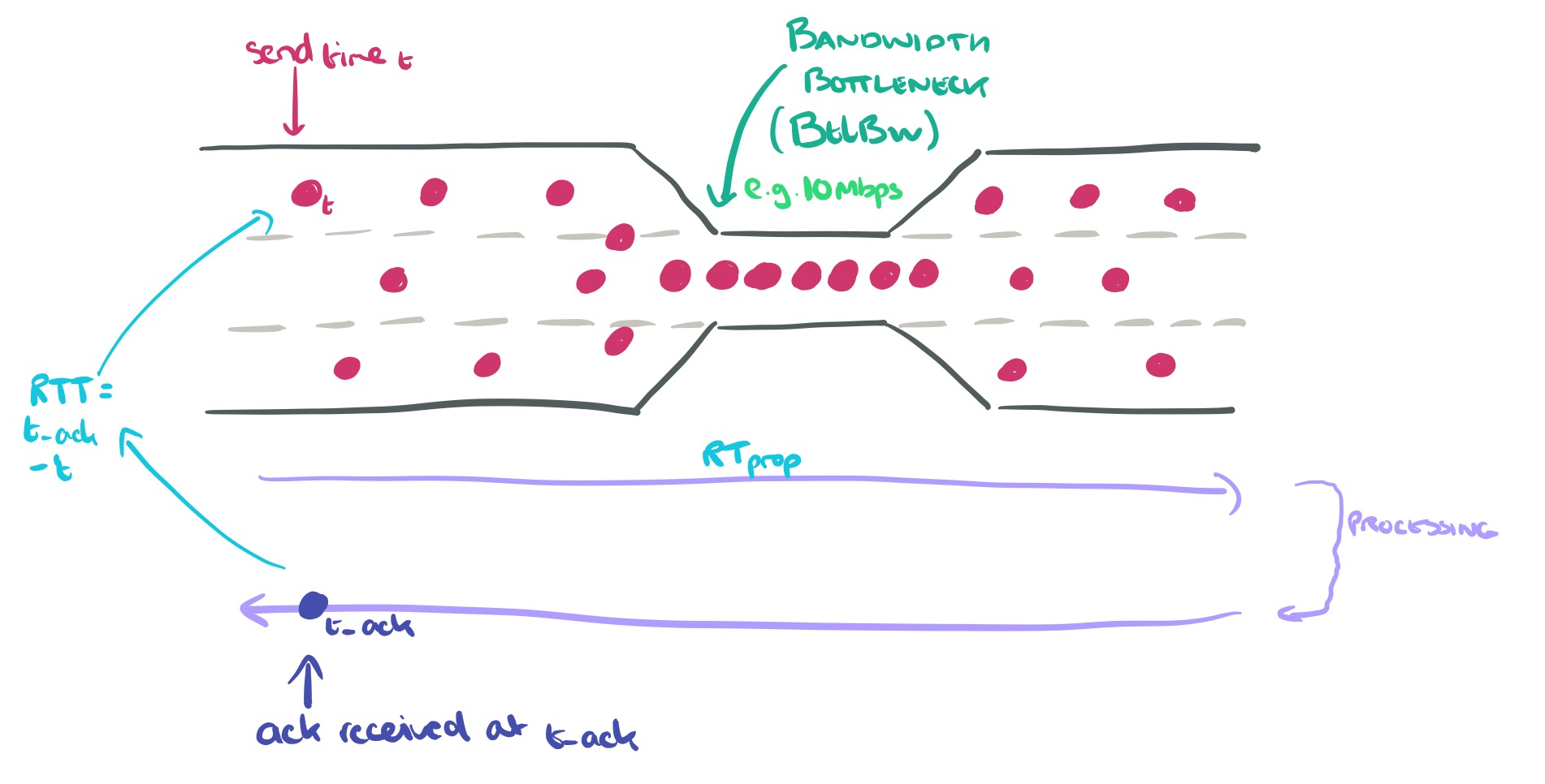
The RTprop time is the minimum time for round-trip propagation if there are no queuing delays and no processing delays at the receiver. The more familiar RTT (round-trip time) is formed of RTprop + these additional sources of noise and delay.
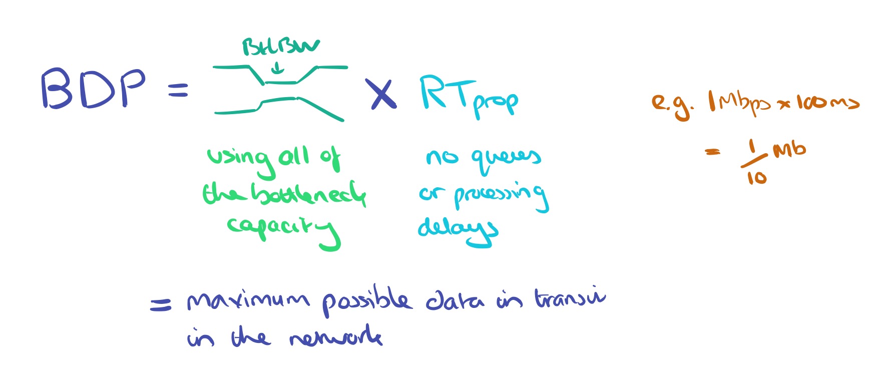
Bandwidth Delay Product (BDP) is the maximum possible amount of data in transit in a network, and is obtained by multiplying the bottleneck bandwidth and round-trip propagation time.
BDP is central to understanding network performance. Consider what happens to delivery rate as we gradually increase the amount of data inflight. When the amount of inflight data is less than BDP, then delivery rate increases as we send more data – delivery rate is limited by the application. Once the bandwidth at the bottleneck is saturated though, the delivery rate cannot go up anymore – we’re pushing data through that pipe just as fast as it can go. The buffer will fill up, eventually we’ll start dropping packets, but we still won’t increase delivery rate.
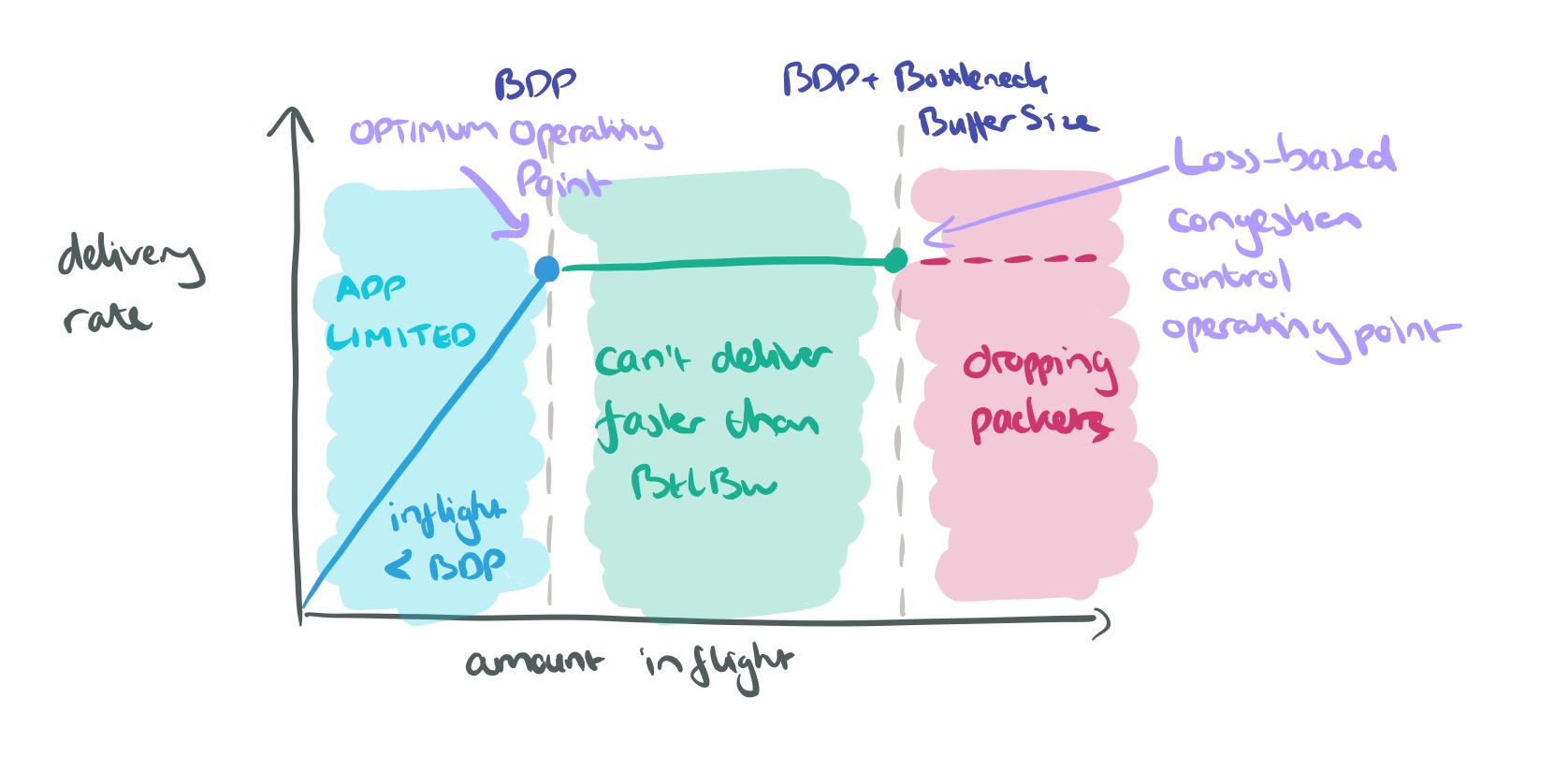
The optimum operating point is right on the BDP threshold (blue dot above), but loss-based congestion control operates at the BDP + Bottleneck Buffer Size point (green dot above).
Now let’s look at what happens to RTT as we increase the amount of data inflight. It can never be better than RTprop, so until we reach BDP, RTT ~= RTprop. Beyond BDP, as buffers start to fill, RTT goes up until buffers are completely full and we start dropping packets.
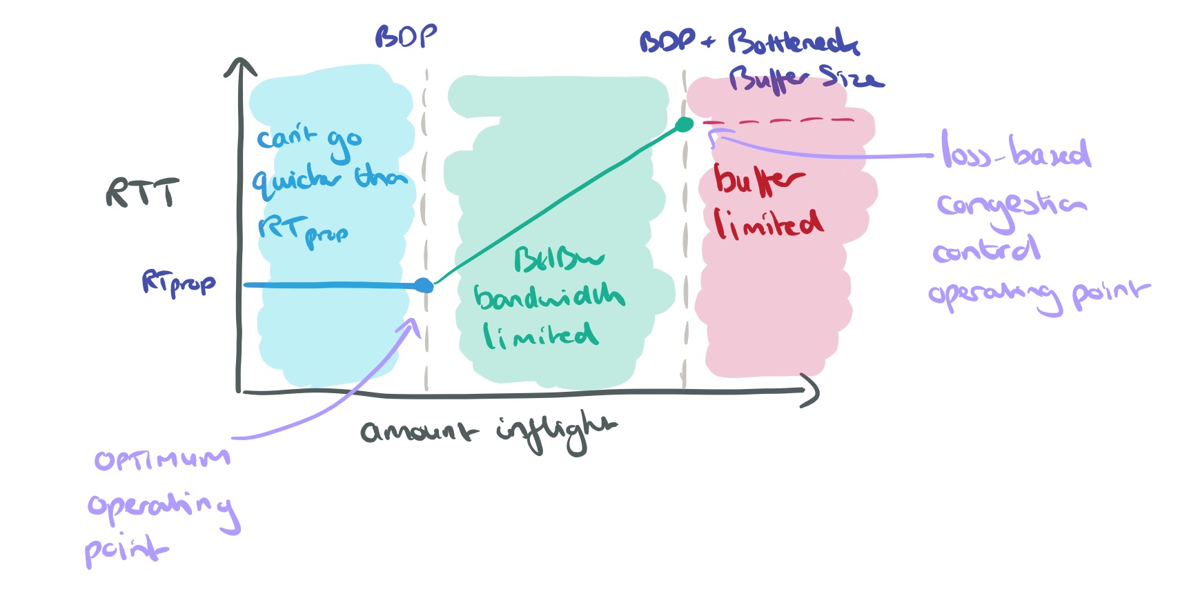
Once more, the optimum operating point would be right on the BDP threshold. This was proved by Leonard Kleinrock in 1979, unfortunately about the same time Jeffrey M. Jaffe proved that it was impossible to create a distributed algorithm that converged to this operation point. Jaffe’s result rests on fundamental measurement ambiguities.
Although it is impossible to disambiguate any single measurement, a connection’s behavior over time tells a clearer story, suggesting the possibility of measurement strategies designed to resolve ambiguity.
Introducing BBR
BBR is a congestion control algorithm based on these two parameters that fundamentally characterise a path: bottleneck bandwidth and round-trip propagation time. It makes continuous estimates of these values, resulting in a distributed congestion control algorithm that reacts to actual congestion, not packet loss or transient queue delay, and converges with high probability to Kleinrock’s optimal operating point.
(BBR is a simple instance of a Max-plus control system, a new approach to control based on nonstandard algebra. This approach allows the adaptation rate [controlled by the max gain] to be independent of the queue growth [controlled by the average gain]. Applied to this problem, it results in a simple, implicit control loop where the adaptation to physical constraint changes is automatically handled by the filters representing those constraints. A conventional control system would require multiple loops connected by a complex state machine to accomplish the same result.)
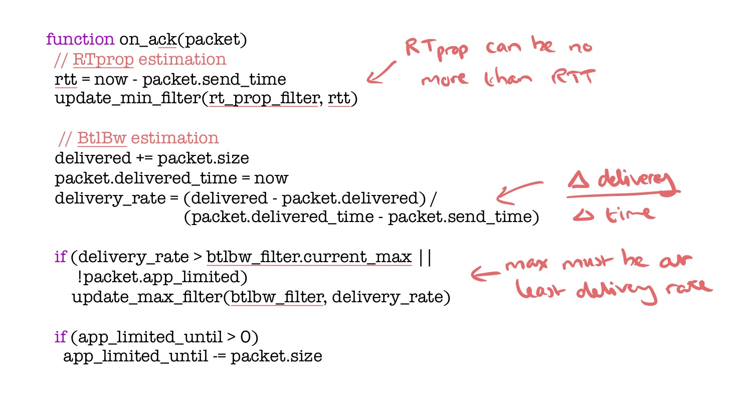
Since RTT can never be less than RTprop, tracking the minimum RTT provides an unbiased and efficient estimator of the round-trip propagation time. The existing TCP acks provide enough information for us to calculate RTT.
Unlike RTT, nothing in the TCP spec requires implementations to track bottleneck bandwidth, but a good estimate results from tracking delivery rate.
The average delivery rate between a send and an ack is simply the amount of data delivered divided by the time taken. We know that this must be less than the true bottleneck delivery rate, so we can use the highest recorded delivery rate as our running estimate of bandwidth bottleneck.
Putting this altogether leads to a core BBR algorithm with two parts: a protocol to follow on receiving an ack, and a protocol to following when sending. You’ll find the pseudocode for these on pages 28 and 29-30. From my reading, there are a couple of small mistakes in the pseudocode (but I could be mistaken!), so I’ve recreated clean versions below. Please do check against those in the original article if you’re digging deeper…
Here’s the ack protocol:
(app_limited_until is set on the sending side, when the app is not sending enough data to reach BDP). This is what the sending protocol looks like:
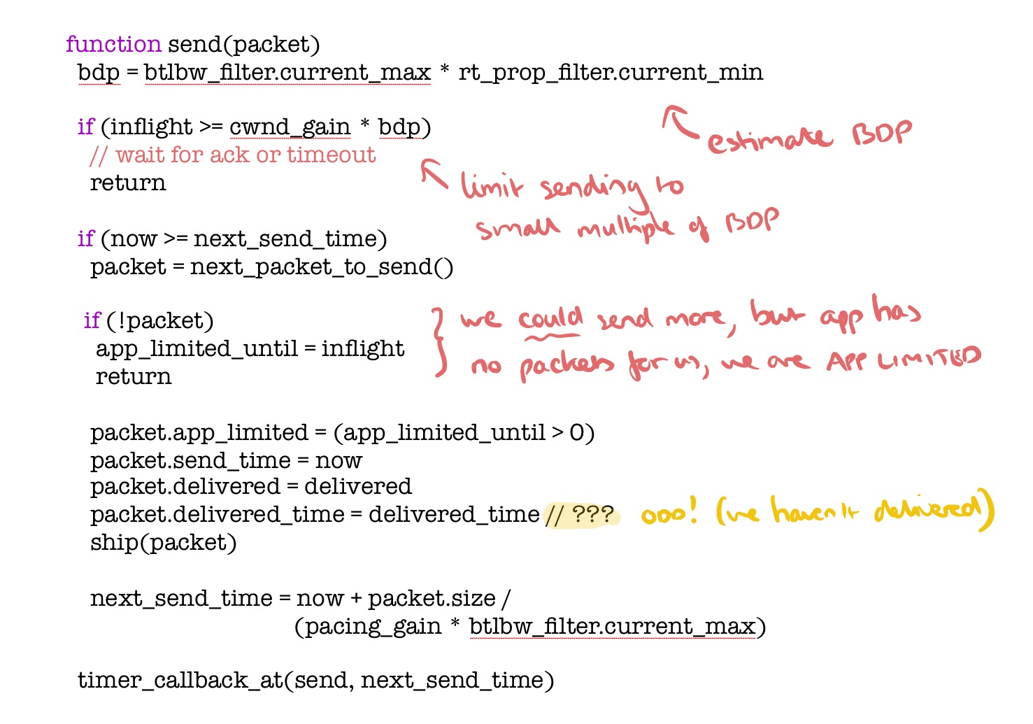
The pacing_gain controls how fast packets are sent relative to BtlBw and is key to BBR’s ability to learn. A pacing_gain greater than 1 increases inflight and decreases packet inter-arrival time, moving the connection to the right on the performance charts. A pacing_gain less than 1 has the opposite effect, moving the connection to the left. BBR uses this pacing_gain to implement a simple sequential probing state machine that alternates between testing for higher bandwidths and then testing for lower round-trip times.
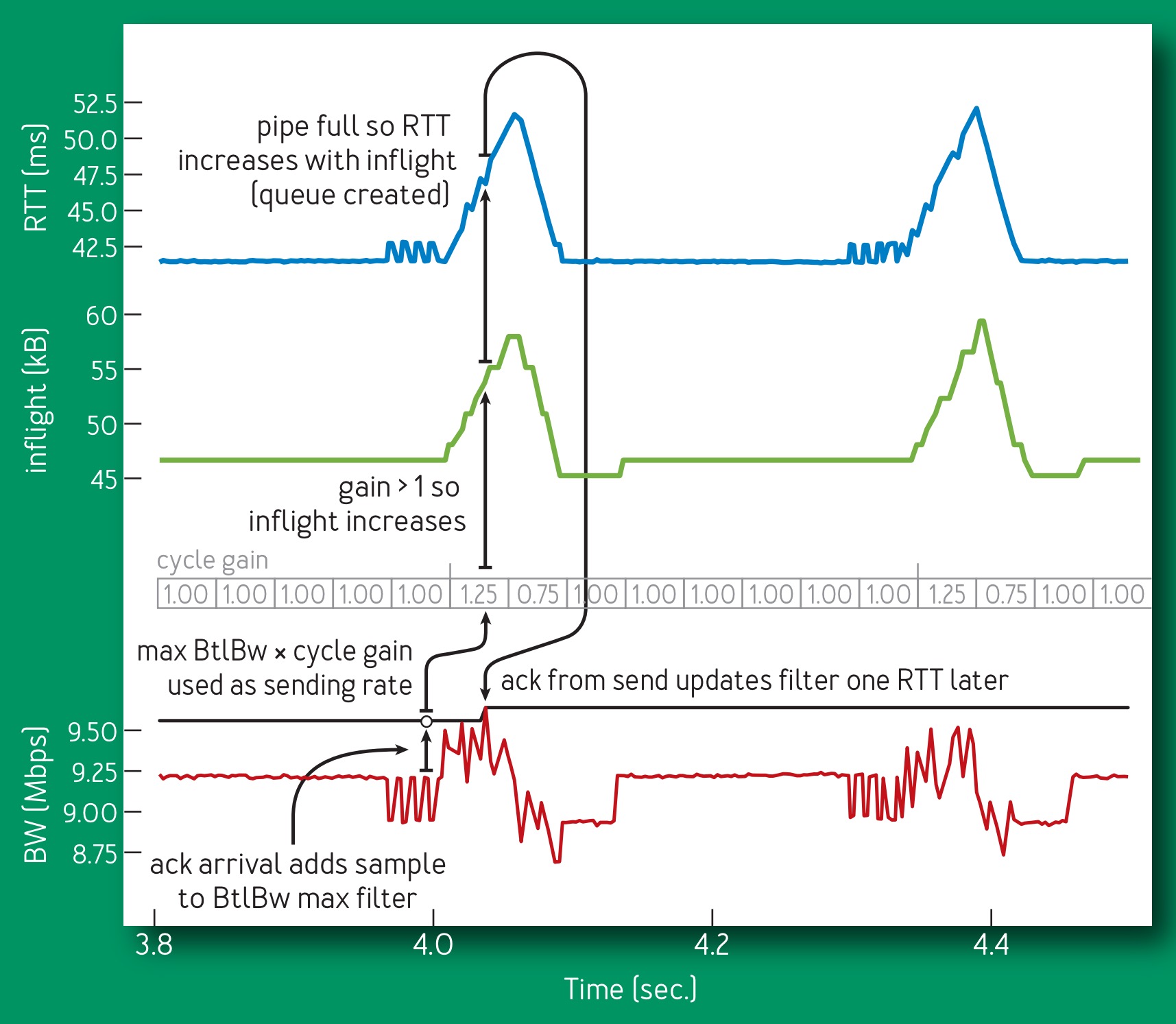
The frequency, magnitude, duration and structure of these experiments differ depending on what’s already known (start-up or steady state) and the sending app’s behaviour (intermittent or continuous). Most time is spent in the ProbeBW state probing bandwidth. BBR cycles through a sequence of gains for pacing_gain, using an eight-phase cycle with values 5/4, 3/4, 1, 1, 1, 1, 1, 1. Each phase lasts for the estimated round-trip propagation time.
This design allows the gain cycle first to probe for more bandwidth with a pacing_gain above 1.0, then drain any resulting queue with a pacing_gain an equal distance below 1.0, and then cruise with a short queue using a pacing_gain of 1.0.
The result is a control loop that looks like this plot below showing the RTT (blue), inflight (green) and delivery rate (red) from 700ms of a 10Mbps, 40-ms flow.
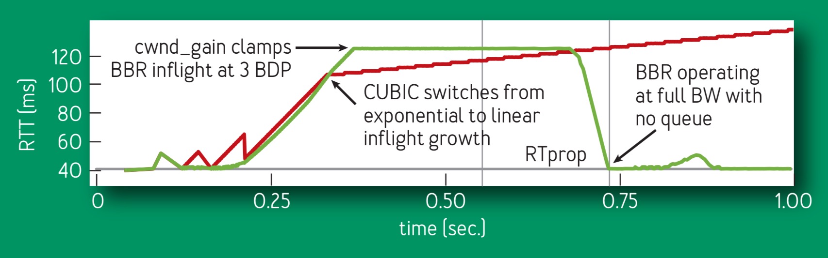
Here’s how BBR compares to CUBIC during the first second of a 10 Mbps, 40-ms flow. (BBR in green, CUBIC in red).
We talked about the BBR benefits in Google’s high-speed WAN network (B4) and in YouTube in the introduction. It also has massive benefits for low bandwidth mobile subscriptions.
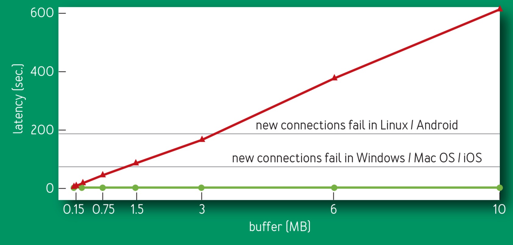
More than half of the world’s 7 billion mobile Internet subscriptions connect via 8-to 114-kbps 2.5 G systems, which suffer well-documented problems because of loss-based congestion control’s buffer-filling propensities. The bottleneck link for these systems is usually between the SGSN (serving GPRS support node)18 and mobile device. SGSN software runs on a standard PC platform with ample memory, so there are frequently megabytes of buffer between the Internet and mobile device. Figure 10 [ below] compares (emulated) SGSN Internet-to-mobile delay for BBR and CUBIC.

There is a related report of better TCP congestion control deployed with a banks data centre https://www.usenix.org/system/files/conference/nsdi15/nsdi15-paper-judd.pdf
Please do an article on the rowhammer exploit
In your on_ack pseudocode, you’ve badly mangled the calculation of deliveryRate. To anyone reading this, refer to the correct code in the original article!
The result is a control loop that looks like this plot below showing the RTT (blue), inflight (green) and delivery rate (red) from 700ms of a 10Mbps, 40-ms flow.
What is the mean 700ms?