Write-limited sorts and joins for persistent memory Viglas, VLDB 2014

This is the second of the two research-for-practice papers for this week. Once more the topic is how database storage algorithms can be optimised for NVM, this time examining the asymmetry between reads and writes on NVM. This is premised on Viglas’ assertion that:

Writes are more than one order of magnitude slower than DRAM, and thus more expensive than reads…

I’ve found it very hard to get consistent data about NVM performance. In yesterday’s paper we find this table which shows equivalent read and write latency for RRAM and MRAM, but 3:1 write:read latency for PCM.

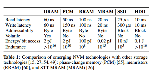
Viglas uses reference points of 10ns for reads and 150ns for writes. 10ns is on the order of an L3 cache read from previous figures I’ve looked at.

Let’s proceed on the assumption that at least in some forms of NVM, there is a material difference between read and write latency. On this basis, Viglas examines algorithms for sorts and joins that can be tuned to vary the ratio of read and write operations. Beyond performance, another reason to reduce writes is to reduce the impact of write degradation over the lifetime of the memory.

All the algorithms work by trading writes for reads. There are two basic approaches:

• Algorithms that partition their input (with a configurable threshold) between a part that is processed by a regular write-incurring strategy, and a part that is processed by a write-limited strategy.
• Algorithms that use lazy processing to defer writes for intermediate results until the cost of recreating them (additional reads + computation) exceeds the cost of the write.

Partitioned Sorting

The partitioned sorting algorithm, called segment sort trades off between a traditional external mergesort and a selection sort.

External mergesort splits the input into chunks that fit in main memory, and sorts each chunk in memory before writing it back to disk (in sorted form) as a run. Runs are then merged in passes to produce the sorted output, the number of passes required being dictated by the available memory.

Selection sort, at a cost of extra reads, writes each element of the input only once at its final location. On each pass it finds smallest set of values that will fit in its memory budget of M buffers, maintains them in eg. a max-heap when sorting in ascending order, and then writes them out as a run at the end of the pass. For an input T buffers in size this algorithm performs |T| . |T|/M read passes and |T| writes.

In segment sort we decide x ∈ (0,1), the fraction of the input that will be sorted using external mergesort (and hence 1-x is sorted using selection sort). Each segment is processed independently using the respectively algorithm, and at the end runs are merged using the standard merging phase of external merge sort.

How do you choose the appropriate value of x? Simple! 😉

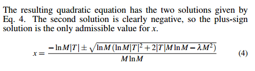
where λ is the read/write ratio w_cost/r_cost.

A variation of segment sort called hybrid sort is also introduced, that draws inspiration from hybrid hash join. See §2.1.2 for details.

Lazy Sorting

The lazy sorting approach is based on selection sort.

Our write-limited sort algorithms, given a budget of M buffers, continuously scan the input to extract the next set of minimum values to be appended to the output; each scan processes the entire input. An alternative would be to extract not only the set of minimum values from the input, but also the set of values that are necessary to produce the next set of minimum values. This is possible to achieve by the lazySort algorithm of Algorithm 2. The algorithm tracks the current iteration (i.e., the number of full scans it has performed so far), the benefit of not materializing the input for the next scan, and the penalty it has paid by rescanning the input. In each iteration the algorithm compares the cost of materializing the next input to the cost of rescanning the current input. If the rescanning cost exceeds the materialization cost, then the algorithm materializes the next input; else it proceeds as before.

Partitioned Joins

For equi-joins, Viglas trades-off between Grace join and standard nested loops joins. The Grace join component issues writes, the nested loops one is read-only. If we’re joining T and V, we need to decide the percentage x of T and the percentage y of V that will be processed using the Grace join.

Viglas offers the following heuristics for setting x and y:

If the inputs are similarly sized andthe medium is not too inefficient then we are better off using large values for x and y, i.e. employing Grace join; this is intuitive as Grace join is more effcient than nested loops. If the inputs have similar sizes then the decisive factor is λ the write to read ratio of the medium. As λ grows the advantage shifts to nested loops. On the other hand, as the ratio between input sizes changes, we can start gradually employing nested loops as the evaluation algorithm.

Segmented Grace join divides the input into partitions and operates at a partition level. It first scans both inputs and offloads k partitions where k is the size of the first input divided by the size of the memory budget available, |T|/M. Given these k partitions, we process x of them with Grace join, and k-x with standard nested loops.

We can be guided by the following equation to choose x , which tells us the conditions under which Grace join is the better choice:

Regardless of outperforming (plain) Grace join, the choice of x is a knob by which we can alter the write intensity of the algorithm.

Lazy hash joins

A standard hash join with two inputs T and V where |T| < |V| computes a join in k = |T|/M iterations by partitioning the inputs into m partitions.

During iteration i the algorithm scans T and hashes each t ∈ T to identify its partition. If t belongs to partition i, the algorithm puts it in an in-memory hash table. If t belongs to any other partition it offloads it to the backing store. The algorithm then scans V and hashes each v ∈ V to identify its partition. If v belongs to partition i it is used to probe the in-memory hash table; any matches are propagated to the output. If t does not belong to partition i, it is offloaded to the backing store. The algorithm iterates as above until both inputs are exhausted. Thus, M buffers from T and M_V = |V|/k buffers from V are eliminated in each iteration.

The lazy version does not write back records it encounters that do not belong to the partition currently being processed. Instead, it pays the penalty of rescanning the input during the next iteration. As before, it will act lazily until the cost of doing so exceeds the costs of the writes, at which point it materializes an intermediate input and the reverts to being lazy again. Lazy hash join needs to materialize these intermediate results every n = k/(λ + 1) iterations.

Persistent memory strategies

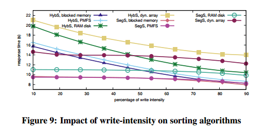
A salient decision to make when incorporating persistent memory into the programming stack is whether to treat it as part of the filesystem, or as part of the memory subsystem. The first option fully addresses the persistence aspects, but implies the traditional boundary between main memory and secondary storage. The second option makes persistent memory part of the memory hierarchy treated as volatile; thus the system itself must guarantee persistence. Our goal is not to answer the question of which option is better. Rather, it is to showcase the performance of our algorithms under each option.

It may not be a goal to answer the question of which option is better, but in the evaluation a clear winner does emerge for these algorithms, blocked memory. In this model the persistent collections implementation on top of which the storage algorithms are layered offers the interface of a dynamic array with byte addressability, but uses a linked list of memory blocks under the covers. Memory is allocated one block at a time.

While array expansion in a main memory setting bears a one-off cost that is dwarfed by the benefits of improved locality, this is no longer the case for persistent memory and its asymmetric write/read costs. Thus, an implementation optimized for main memory is not the best choice for persistent memory. Treating persistent memory as block-addressable storage albeit mounted in main memory is not the best option either as it introduces significant overhead. A persistent collection implementation based on blocked memory shows the true potential of the hardware and the algorithms as it effectively bears zero overhead apart from the unavoidable penalties due to the write/read cost asymmetry.

Performance analysis

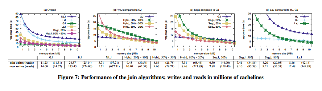
The analysis compares four sort variations and six join variations, identified in the graphs as:

Sorting:

1. ExMS – standard external mergesort
2. SegS – segment sort (which trades between external mergesort and selection sort)
3. HybS – the hybrid sort variation of segment sort
4. LaS – lazy sort

Joining:

1. GJ – standard Grace join
2. HS – simple hash join
3. NLJ – nested loops join
4. HybJ – Hybrid Grace-nested-loops join
5. SegJ – segmented Grace join
6. LaJ – lazy join

(Click for larger view)

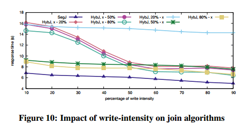
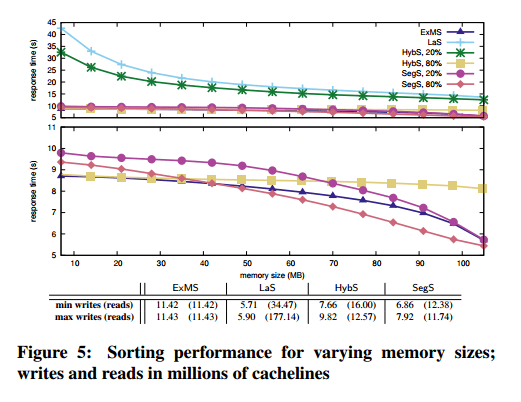
The results affirm that choosing algorithms or implementations when incorporating persistent memory into the I/O stack is not straightforward. It is a combination of various parameters and it comes down to what we want to optimize for. The algorithms do well in introducing write intensity and giving the developer, or the runtime, a knob by which they can select whether to minimize writes; or minimize response time; or both. It is also important that the majority of algorithms converges to I/O-minimal behavior at a low write intensity; e.g., SegS and SegJ approximate or outperform their counterparts optimized for symmetric I/O from a 20% write intensity onwards. This confirms that one can have write-limited algorithms without compromising performance.