Context-Dependent Pre-Trained Deep Neural Networks for Large-Vocabulary Speech Recognition – Dahl et al. 2011

The title may be a bit of a mouthful, but this paper is often cited as a watershed moment for deep learning and speech recognition. It represents the first application of deep neural networks for large vocabulary speech recognition (LVSR), and the resulting system significantly outperformed the previous state of the art. It uses several of the ideas we saw yesterday including the use of unsupervised pre-training followed by supervised learning, and hierarchies of abstractions.

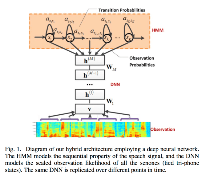
Hidden Markov Models (HMMs) have been the dominant technique for LVSR for at least two decades. An HMM is a generative model in which the observable acoustics features are assumed to be generated from a hidden Markov process that transitions between states S = {s₁,…,s_K}… In conventional HMMs used for automatic speech recognition, the observation properties are modeled using Gausian Mixture Models (GMMs). These GMM-HMMs are typically trained to maximize the likelihood of generating the observed features.

The authors combine a deep neural network (DNN) and HMM. The DNN is pre-trained to predict a distribution over senones using unsupervised learning. Once this pre-training is complete, the weights are retained but otherwise the pre-training DNN is abandoned and (supervised) training continues using backpropagation.

So what’s a senone? There’s a helpful description in the CMUSphinx tutorial: http://cmusphinx.sourceforge.net/wiki/tutorialconcepts. A phone is a class of sound in speech. A triphone is a phone considered in context with its left and right phones. For example the b-a-d in the word ‘bad’ sounds a bit different from the b-a-n in the word ‘ban’. A detector for a part of a triphone (e.g. the beginning) may be shared across many triphones, and is called a senone.

In this paper, we use the DBN (Deep Belief Network) weights resulting from the unsupervised pre-training algorithm to initialize the weights of a deep, but otherwise standard, feed-forward neural network and then simply use the backpropagation algorithm to fine-tune the network weights with respect to a supervised criterion. Pre-training followed by stochastic gradient descent is our method of choice for training deep neural networks because it often outperforms random initialization for the deeper architectures we are interested in training and provides results very robust to the initial random seed. The generative model learned during pre-training helps prevent overfitting, even when using models with very high capacity and can aid in the subsequent optimization of the recognition weights.

The big picture works as follows:

• First, train a traditional context-dependent, Gaussian mixture model, hidden Markov model (CD-GMM-HMM). Give each senone in the model a unique senoneid, and generate a mapping from each physical tri-phone state to the corresponding senoneid.
• Convert this model to a CD-DNN-HMM using the tri-phone and senone structure as well as the transition probabilities from the CD-GMM-HMM.
• Pre-train each layer in the DNN bottom-up by layer (described below).
• Conduct rounds of supervised training until no further improvement in recognition accuracy is observed in the development set: (i) use the tri-phone state to senoneid mapping to fine-tune the DNN using backpropagation; (ii) estimate the prior probability of each senone simply based on the percentage of frames it appears in; (iii) re-estimate the transition probabilities to maximize the likelihood of observing the features (using the pre- and post- states of the DNN for this round of supervised learning); (iv) generate a new state mapping for the training set based on the new network.

The results are evaluated on a business search dataset collected from the Bing mobile voice search application in 2008. The training set comprised 24 hours of audio, and 32,057 utterances. The development set comprised 6.5 hours of audio, and 8,777 utterances. The test set comprised 9.5 hours of audio and 12,758 utterances. Performance was evaluated using sentence accuracy instead of word accuracy (sentences in this dataset are quite short, at 2.1 tokens on average).

Overall, our proposed CD-DNN-HMMs obtained 69.6% accuracy on the test set, which is 5.8% (or 9.2%) higher than those obtained using the minimum phone error (MPE) or maximum likelihood (ML) trained CD-GMM-HMMs. This improvement translates to a 16.0% (MPE) or 23.2% (ML) relative error-rate reduction and is statistically significant at a significant level of 1% according to McNemar’s test.

The authors conducted experiments to see how sentence accuracy improves as more layers are added in the CD-DNN-HMM.

When three hidden layers were used, the accuracy increased to 69.6%. The accuracy further improved to 70.2% with four hidden layers and 70.3% with five hidden layers. Overall, using the five hidden-layer models provides us with a 2.2% accuracy improvement over a single hidden-layer system when the same alignment is used. Although it is possible that using even more than five hidden layers would continue to improve the accuracy, we expect any such gains to be modest at best, so we restricted ourselves to at most five hidden layers in the rest of this work…

Pre-training a Deep Belief Network

Deep belief networks (DBNs) are probabilistic generative models with multiple layers of stochastic hidden units above a single bottom layer of observed variables that represent a data vector. DBNs have undirected connections between the top two layers and directed connections to all other layers from the layer above. There is an efficient unsupervised algorithm, first described in [24], for learning the connection weights in a DBN that is equivalent to training each adjacent pair of layers as an restricted Boltzmann machine (RBM)…

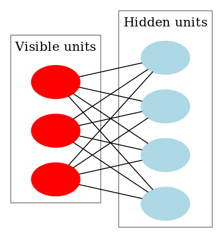
Restricted Boltzmann machines are constructed from a layer of binary stochastic hidden units and a layer of stochastic visible units.

(Image from wikipedia)

A traditional RBM dealing with binary units assigns an energy to every configuration of visible v and hidden h state vectors. This energy has three terms:

E(v,h) = –b^Tv – c^Th – v^TWh

where b is a visible unit bias, c is a hidden unit bias, and W is the matrix of connection weights between the visible and hidden components. The probability of any particular setting of the hidden and visible units is a function of the energy of that configuration. After some simplification, it turns out that the probability a hidden unit is set to 1 is given by:

P(h=1|v) = σ(c + v^TW) (7)

where σ is the elementwise logistic sigmoid function, _σ(x) = (1 + e^-x)^-1.

The form of P(h=1|v) is what allows us to use the weights of an RBM to initialize a feed-forward neural network with sigmoidal hidden units because we can equate the inference for RBM hidden units with forward propagation in a neural network.

Speech data has real-valued feature vectors as opposed to binary inputs. The Guassian-Bernoulli restricted Boltzmann machine (GRBM) enables RBMs to work with real-valued data, using a modified energy function:

E(v,h) = ½(v – b)^T(v – b) – c^Th – v^TWh

An RBM is trained using stochastic gradient descent on the negative log likelihood. This gradient is not feasible to compute exactly, but an approximation can be used.

Since RBMs are in the intersection between Boltzmann machines and product of experts models, they can be trained using contrastive divergence as described in [67]…

Once an RBM is trained on data, we can use equation (7) to compute a vector of hidden unit activation probabilities h for each data vector v. These can be used as training data for a new RBM…

Thus, each set of RBM weights can be used to extract features from the output of the previous layer. Once we stop training RBMs, we have the initial values for all the weights of the hidden layers of a neural net with a number of hidden layers equal to the number of RBMs we trained. With pre-training complete, we add a randomly initialized softmax output layer and use backpropagation to fine-tune all the weights in the network discriminatively.

In conclusion

We have described a context-dependent DNN-HMM model for LVSR that achieves substantially better results than strong, discriminatively trained CD-GMM-HMM baselines on a challenging business search dataset. Although our experiments show that CD-DNN-HMMs provide dramatic improvements in recognition accuracy, training CD-DNN-HMMs is quite expensive compared to training CD-GMM-HMMs (although on a similar scale as other neural-network based acoustic models and certainly feasible for large datasets, if one can afford weeks of training time)… Finding new ways to parallelize training may require a better theoretical understanding of deep learning.