Trajectory Data Mining: An Overview – Zheng 2015

In ‘Trajectory Data Mining,’ Zheng conducts a high-level tour of the techniques involved in working with trajectory data. This is the data created by a moving object, as a sequence of locations, often with uncertainty around the exact location at each point. This could be GPS trajectories created by people or vehicles, spatial trajectories obtained via cell phone tower IDs and corresponding transmission times, the moving trajectories of animals (e.g. birds) fitted with trackers, or even data concerning natural phenomena such as hurricanes and ocean currents. It turns out there’s a lot to learn about working with such data! Here’s a map of the territory covered in the paper:

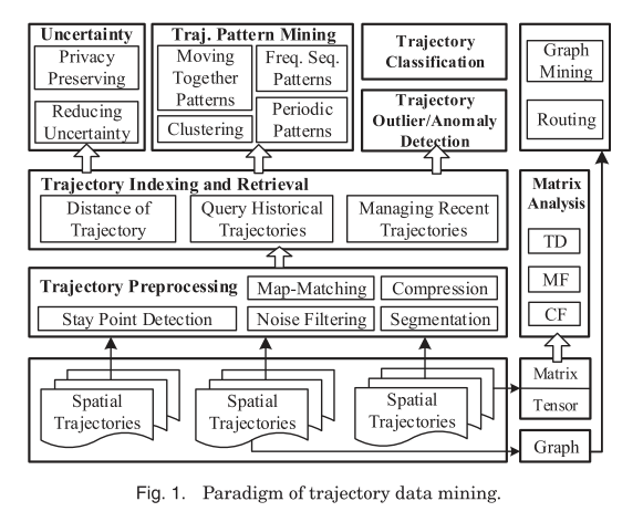
Trajectory Preprocessing is concerned with cleaning up the data to prepare for higher-level processing. Trajectory Indexing and Retrieval describes data structures that support efficient indexing and retrieval of trajectory information (for example, nearest neighbours and range queries). Trajectory Pattern Mining looks for trajectories following certain patterns, or groups of similar trajectories. Trajectory Classification is the art of labelling trajectory segments with additional data – typically the likely mode of transport (walking, cycling, driving etc.). I’m going to concentrate of these four areas in this write-up (and even then, I’m skipping a lot of detail, the full paper runs to 41 pages). For further details such as how to convert trajectories into graph, matrix, and tensor forms for additional analysis I refer you to the paper.

Trajectory Preprocessing

Noise Filtering

Spatial trajectories have noise in them – locations can be off by several hundred meters or more depending on the technology used and the physical conditions at the true location (e.g. urban canyons). For some applications, such as determining travel speed, this can be an issue. For isolated noisy points, a mean (or median) filter can be used. This works by estimating the true location of a point using a sliding window of n values and taking the mean / median. With a low sampling rate of trajectory though this method does not work so well. In that case we might turn to a Kalman filter or particle filter that includes estimates of motion.

Besides giving estimates that obey the laws of physics, the Kalman filter gives principled estimates of higher order motion states like speed. While the Kalman filter gains efficiency by assuming linear models plus Gaussian noise, the particle filter relaxes these assumptions for a more general, but less efficient, algorithm.

These filters are sensitive to the initial location in a trajectory – if this is also noisy then effectiveness is reduced. In this circumstance, a third approach is to use outlier detection algorithms based on some combination of velocity and distance.

Stay points

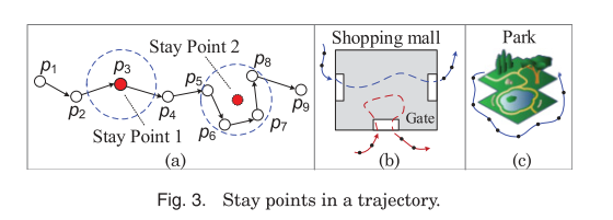
Once noise is removed, another common task is the detection of stay points – points in the spatial trajectory where the object being tracked paused for some time. Even if the measured object actually stays stationary, the position readings are likely to move around. Determining stay points enables us to transform a sequence of locations into a sequence of meaningful places visited.

Li et al. [2008] first proposed the stay point detection algorithm. This algorithm first checks if the distance between an anchor point (e.g., p5) and its successors is in a trajectory larger than a given threshold (e.g., 100 m). It then measures the time span between the anchor point and the last successor (i.e., p8) that is within the distance threshold. If the time span is larger than a given threshold, a stay point (characterized by p5, p6, p7, and p8) is detected; the algorithm starts detection of the next stay point from p9. Yuan et al. [2011b, 2013b] improved this stay point detection algorithm based on the idea of density clustering. After finding p5 to p8 is a candidate stay point (using p5 as an anchor point), their algorithm further checks the successor points from p6. For instance, if the distance from p9 to p6 is smaller than the threshold, p9 will be added into the stay point.

Compression

Especially for bandwidth or power-constrained applications, we may want to compress an online trajectory in order to send less data.

As many applications require one to transmit trajectory data in a timely fashion, a series of online trajectory compression techniques have been proposed to determine whether a newly acquired spatial point should be retained in a trajectory. There are two major categories of online compression methods. One is the window-based algorithms, such as the Sliding Window algorithm [Keogh et al. 2001] and Open Window algorithm [Maratnia and de By 2004]. The other is based on the speed and direction of a moving object… For instance, Potamias et al. [2006] use a safe area, derived from the last two locations and a given threshold, to determine whether a newly acquired point contains important information.

Segmentation

Segmentation is the process of dividing a trajectory up into parts (segments).

The segmentation not only reduces the computational complexity but also enables us to mine richer knowledge, such as subtrajectory patterns, beyond what we can learn from an entire trajectory.

There are three general types of segmentation methods:

1. Based on time intervals
2. Based on the shape of the trajectory (e.g. looking for turning points where the heading direction changes over some threshold)
3. Based on semantic meaning of the segments. For example, based on the kinds of stay points, or the estimated mode of transport (walk segments vs drive segments etc.).

Map-matching

Map matching is a process to convert a sequence of raw latitude/longitude coordinates to a sequence of road segments. Knowledge of which road a vehicle was/is on is important for assessing traffic flow, guiding the vehicle’s navigation, predicting where the vehicle is going, and detecting the most frequent travel path between an origin and a destination, and so forth. Map matching is not an easy problem, given parallel roads, overpasses, and spurs [Krumm 2011]. There are two approaches to classify map matching methods, based on the additional information used, or the range of sampling points considered in a trajectory.

• Geometric algorithms consider the actual shape of roads in a road network – for example matching GPS points to the nearest road segment.
• Topological algorithms take into account the actual connectivity of a road network. For example, using the Frechet distance to measure the fit between a GPS sequence and candidate road sequence [Brakatsouls et al. 2005].
• Probabilistic algorithms deal with noisy and low-sampling rate conditions and consider multiple possible paths through a road network to find the most likely one.
• Other advanced algorithms:

More advanced map-matching algorithms have emerged recently that embrace both the topology of the road network and the noise in trajectory data, exemplified by Lou et al. (2009), Newson and Krumm [2009], and Yuan et al. [2010b]. These algorithms find a sequence of road segments that simultaneously come close to the noisy trajectory data and form a reasonable route through the road network.

Trajectory Indexing and Retrieval

There are two major types of queries we want to support over trajectory data: range queries and K-Nearest-Neighbour (KNN) queries:

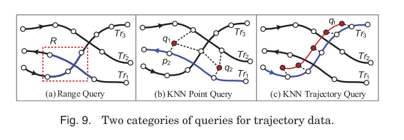
Range queries retrieve the trajectories falling into (or intersecting) a spatial (or spatio-temporal) range. For example, as shown in Figure 9(a), a range query can help us retrieve the trajectories of vehicles passing a given rectangular region R between 2pm and 4pm in the past month. The retrieved trajectories (or segments) can then be used to derive features, such as the travel speed and traffic flow, for data mining tasks like classification and prediction.

Figure 10 below shows the three main structures used for supporting range queries: 3D-Rtrees where time is the third dimension; dividing a time period into multiple time intervals and using an individual spatial index such as an R-tree for the trajectories in each interval; and dividing a geographical space into grids, and then creating a temporal index for the trajectories falling within each grid.

KNN queries retrieve the top-K trajectories with the minimum aggregate distance to a few points (entitled the KNN point query [Chen et al. 2010; Tao et al. 2002; Tang et al. 2011]) or a specific trajectory (entitled the KNN trajectory query [Yi et al. 1998;Agrawal et al. 1993])… To answer such a query, the first step is to define a similarity/distance function between two trajectories. Then efficient query processing algorithms are designed to address the problem of searching over a large set of candidate trajectories.

One distance measure for trajectory segments is based on minimum bounding rectangles. Longest Common Subsequence (LCSS) and Edit Distance (both concepts borrowed from string matching) can also be applied.

Path Inference

Different from the aforementioned models aiming at the retrieval of existing trajectories by different queries, a new series of techniques infers (or say “constructs”) the most likely k route(s) that a moving object could travel (i.e., the missing subtrajectory) between a few sample points based on a bunch of uncertain trajectories. The major insight is that trajectories sharing (or partially sharing) the same/similar routes can often supplement each other to make themselves more complete. In other words, it is possible to interpolate an uncertain trajectory by cross-referring other trajectories on (or partially on) the same/similar route. That is “uncertain + uncertain → certain.” For example, given the uncertain trajectories of many taxicabs (marked by different colored points in Figure 13(a)), we could infer that the blue path is the most likely route traversing (p1,p2,p3).

Trajectory Pattern Mining

Finding things that move together

Here the goal is to find a groups of objects that move together for a certain time period. The literature talks about flocks, swarms, traveling companions_ and gatherings. A flock is a group of objects that travel together within a disk of some user-specified size for at least k timestamps. If the circular shape of the disk is not a good fit to the shape of the group in practice though you may miss flock members.

To avoid rigid restrictions on the size and shape of a moving group, the convoy is proposed to capture generic trajectory patterns of any shape by employing density-based clustering. Instead of using a disk, a convoy requires a group of objects to be density connected during k consecutive time points.

A swarm is like a flock or convoy, but relaxes the requirement that the k time points be consecutive. The traveling companion algorithm finds convoy or swarm-like patters from trajectories that are being streamed into a system (vs. an after-the-fact batch analysis).

To detect some incidents such as celebrations and parades, in which objects join and leave an event frequently, the gathering pattern further loosens the constraints of the aforementioned patters by allowing the membership of a group ot evolve gradually…

Finding common paths taken by many objects

Also known as trajectory clustering.

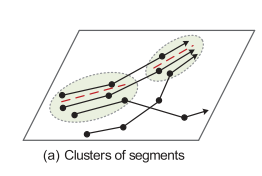
A general clustering approach is to represent a trajectory witha feature vector, denoting the similarity between two trajectories by the distance between their feature vectors. However, it is not easy to generate a feature vector with uniform length for different trajectories…

Trajectories are partitioned into line segments, and groups of close trajectory segments can be found using the Trajectory-Hausdorff Distance. A representative path is then found for each cluster of segments.

A Micro-and-Macro Clustering Framework approach (first used to cluster data streams by Aggarwal et al.) is used in which you first find microscluster of trajectory segment, and then group microclusters into macroclusters.

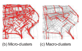
A major insight of Li’s work is that new data will only affect the local area where the new data were received rather than the faraway areas.

Finding sequential patterns

A sequential pattern is a certain number of objects traveling a common sequence of locations in a similar time interval. For example, trajectory A might visit locations L1 → L2 → L7 → L4, and trajectory B might visit locations L1 → L2 → L4. These both share the common sequence L1 → L2 → L4 even though L2 → L4 is not consecutive in A.

When the occurence of such a common sequence in a corpus, usually called support, exceeds a threshold, a sequential trajectory pattern is detected. Finding such patterns can benefit travel recommendation, life pattern understanding, next location prediction, estimating user similarity, and trajectory compression.

Points from different trajectories can be clustered into regions of interest. A point from a trajectory is then represented by the cluster ID the point belongs to, and a trajectory can be re-formed as a sequence of cluster IDs, which can them be compared among different trajectories. Alternatively, we can first detect stay points in a trajectory and then turn a trajectory into a sequence of stay points. In a road-network setting map matching can be used to turn a trajectory into a sequence of road segment IDs. Some sequential pattern mining algorithms such as LCSS and Suffix Tree, designed for strings, can be adapted to find sequential trajectory patterns. Simply take the list of road segments, e.g. r1,r2,r3 and make the string “r1r2r3” …

Finding periodic patterns

Moving objects usually have periodic activity patterns. For example, people go shopping every month and animals migrate yearly from one place to another. Such periodic behaviors provide an insightful and concise explanation over a long moving history, helping compress trajectory data and predict the future movement of a moving object. Periodic pattern mining has been studied extensively for time series data… Due to the fuzziness of spatial locations, existing methods designed for time series data are not directly applicable to trajectories.

Li et al. proposed a two-stage detection method. Firstly a density based clustering algorithm is used to detect reference spots a moving object has visited frequently. Then the trajectory of a moving object is transformed into several binary time series, each of which indicates the “in” (1) or “out” (0) status of the moving object at a reference spot.

Through applying Fourier transform and autocorrelation metods to each time series, the values of periods at each reference spot can be calculated…

The second stage summarises the periodic behaviours from partial movement sequences using a hierarchical clustering algorithm.

Trajectory Classification

In general, trajectory classification is comprised of three major steps: (1) Divide a trajectory into segments using segmentation methods. Sometimes, each single point is regarded as a minimum inference unit. (2) Extract features from each segment (or point). (3) Build a model to classify each segment (or point). As a trajectory is essentially a sequence, we can leverage existing sequence inference models, such as Dynamic Bayesian Network (DBN), HMM, and Conditional Random Field (CRF), which incorporate the information from local points (or segments) and the sequential patterns between adjacent points (or segments).

We might for example classify segments as still or moving, or we could get more sophisticated…

Zhu et al. [2011] aim to infer the status of a taxi, consisting of Occupied, Nonoccupied, and Parked, according to its GPS trajectories. They first seek the possible Parked places in a trajectory, using a stay point-based detection method. A taxi trajectory is then partitioned into segments by these Parked places. For each segment, they extract a set of features incorporating the knowledge of a single trajectory, historical trajectories of multiple taxis, and geographic data like road networks and Points of Interest (POIs). After that, a two-phase inference method is proposed to classify the status of a segment into either Occupied or Nonoccupied. The method first uses the identified features to train a local probabilistic classifier and then globally considers travel patterns via a hidden semi-Markov model.

Classifying a trajectory by transportation modes (e.g. walking, biking, bus, driving) is another common goal.