Understanding hidden memories of recurrent neural networks Ming et al., VAST’17
Last week we looked at CORALS, winner of round 9 of the Yelp dataset challenge. Today’s paper choice was a winner in round 10.
We’re used to visualisations of CNNs, which give interpretations of what is being learned in the hidden layers. But the inner workings of Recurrent Neural Networks (RNNs) have remained something of a mystery. RNNvis is a tool for visualising and exploring RNN models. Just as we have IDEs for regular application development, you can imagine a class of IMDEs (Interactive Model Development Environments) emerging that combine data and pipeline versioning and management, training, and interactive model exploration and visualisation tools.
Despite their impressive performances, RNNs are. still “black boxes” that are difficult for humans to understand… the lack of understanding of how RNN models work internally with their memories has limited researchers’ ability to introduce further improvements. A recent study also emphasized the importance of interpretability of machine learning models in building user’s trust: if users do not trust the model, they will not use it.
The focus of RNNvis is RNNs used for NLP tasks. Where we’re headed is an interactive visualisation tool that looks like this:
(Enlarge)
The source code for RNNvis is available on GitHub at myaooo/RNNvis.
RNN refresher
A ‘vanilla’ recurrent neural network takes a sequence of inputs }")

}")
}")
} = f(\mathbf{Wh}^{(t-1)} + \mathbf{Vx}^{(t)})")


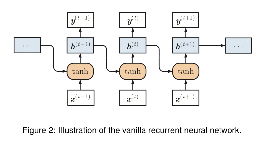
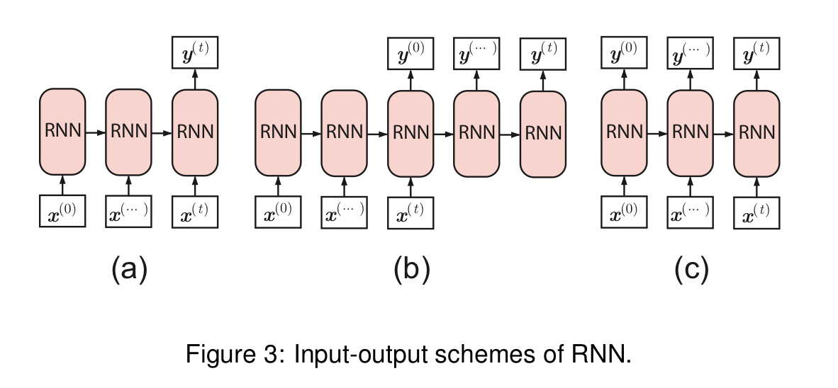
Different models use the outputs
Two common RNN variants are long short-term memory (LSTM) networks and Gated Recurrent Units (GRUs). There are nice succinct explanations of these in Appendix A of the paper.
Challenges and requirements for a visualisation tool
There may be hundreds of thousands of hidden state units storing information extracted from potentially long input sequences. As well as their sheer number, the complex sequential rules embedded in text sequences are intrinsically difficult to interpret and analyse. It also turns out that there is a complex many-to-many relationship between input words and hidden states: each input word generally results in changes in nearly all hidden state units, and each hidden state unit may be highly responsive to multiple words.
In order to provide intuitive interpretations of RNN hidden states to help in diagnosis and improving model designs, we have the following requirements:
- Provide a clear interpretation of the information captured by hidden states (bearing in mind that most interpretable information is distributed across multiple hidden state units)
- Show the overall information distribution across hidden states – how is stored information differentiated and correlated across states?
- Explore hidden state mechanisms at the sequence level
- Examine the detailed statistics of individual states
- Compare the learning outcomes of different models. What makes one model better than another?
RNNvis overview
RNNvis has three major components: a model manager which uses TensorFlow to build, train, and test RNN models; an evaluator which analyses trained models to extract and interpret learned representations; and a visualizer to present the information visually and interactively to the end user.
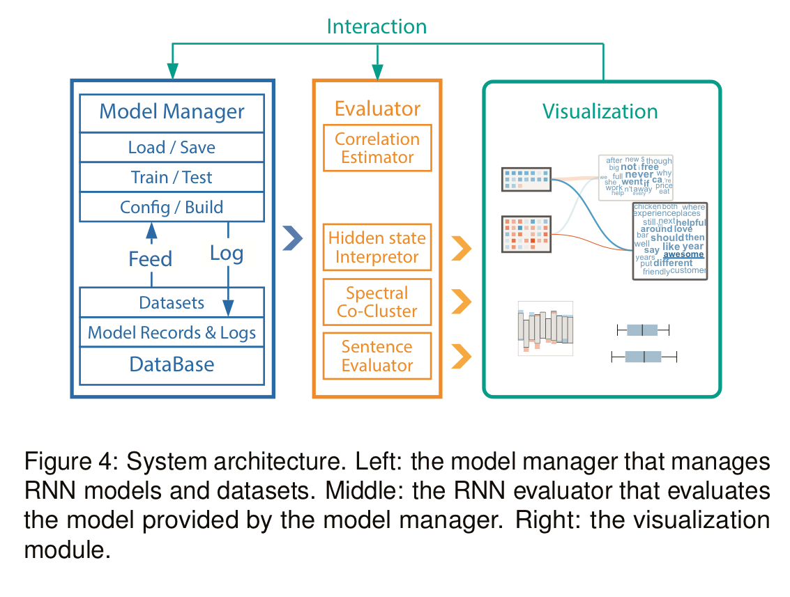
How RNNvis works: model evaluation and interpretation
There are three layers to the model interpretation: interpreting individual hidden states; interpreting the relationships between input words and hidden states as a group; and understanding the response to input sequences.
Individual hidden states
To understand individual hidden states, RNNvis examines the contribution of the output of the hidden state to the overall model output (e.g., a probability distribution over classes), and the change in the hidden state in response to an input word. The response may of course depend upon the sequence history (that’s the whole point of an RNN after all!).
Consequently, we formulate
as a more stable measure of the word’s importance on hidden state units.
The overall explanation of a hidden state unit is formulated as the the m words with the top absolute expected responses.
The relationship between hidden states and words
There are too many words and hidden units to meaningfully show all of their individual interactions. But as just described we do know the top m words for each hidden unit. These relationships between words and hidden units are modelled as edges in a bipartite graph where the nodes are words and hidden units. Co-clustering, aka bipartite graph partitioning, is then used to cluster and structure the hidden state space and word space. The output of this step is a set of word clusters and a set of hidden state clusters, with relationships between theses two cluster types.
Sequences
Sequence activity is evaluated at the cluster level, capturing the extent to which a given cluster of hidden units is positively or negatively activated at a given time step.
How RNNvis works: model visualisation
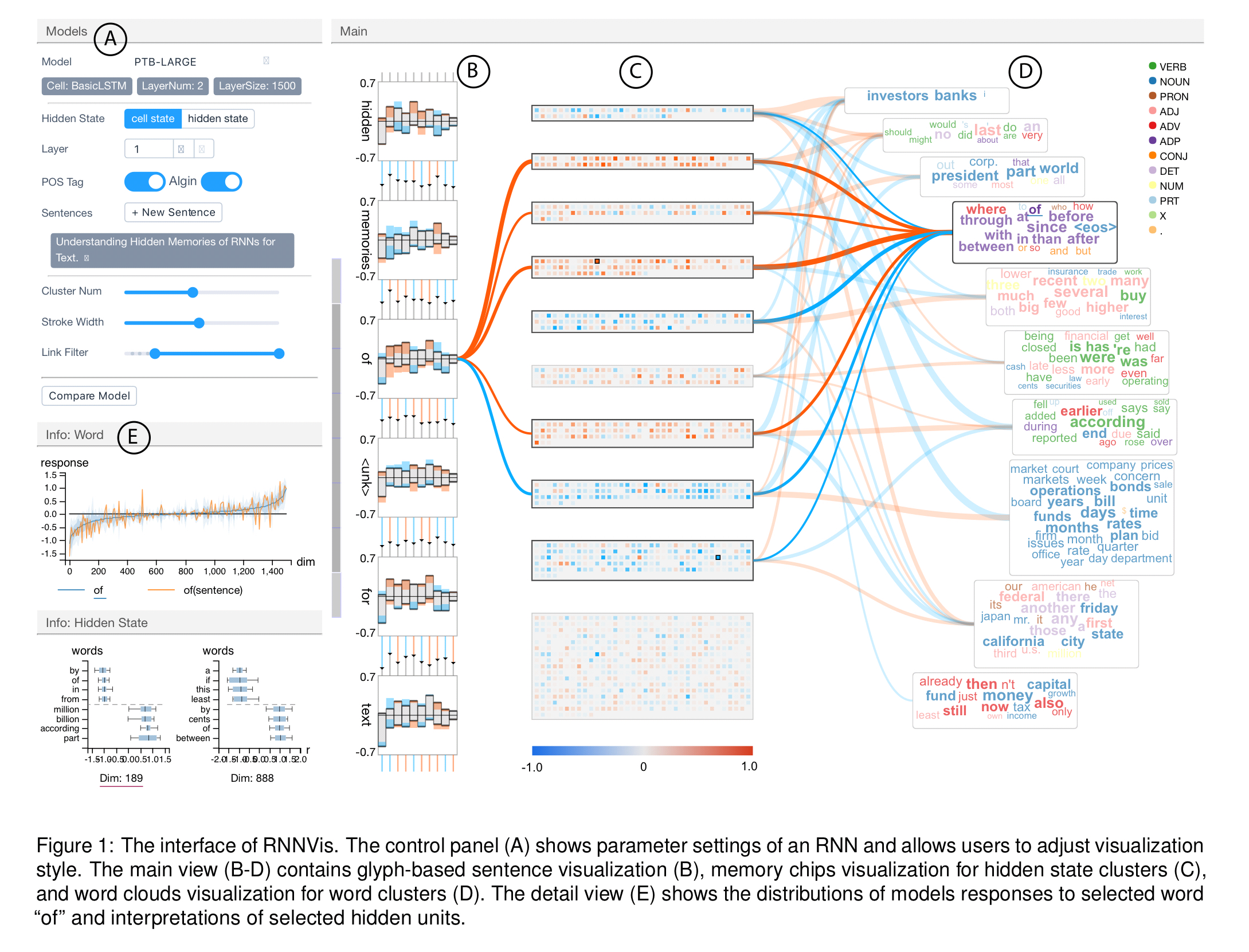
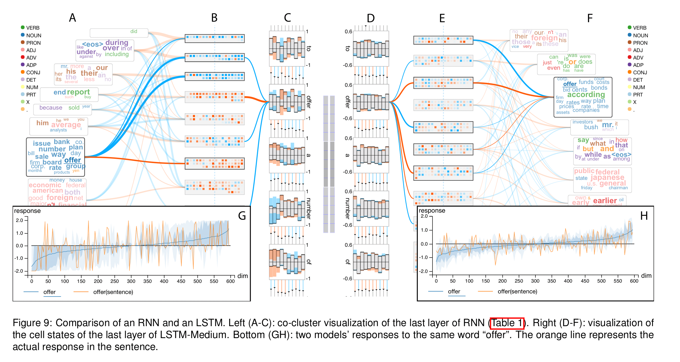
The main RNN visualisation is comprised of three parts (marked B, C, and D in figure 1 at the top of this post).
The set of input words in the sequence are laid out top to bottom on the LHS (column B). For each word there’s a glyph representing the network state after the input of that word. Each bar in the glyph represents a hidden state cluster, split by the horizontal line into positive and negative contributions. At each step the orange colour is used to encode an increase in positive information (or decrease in negative), and the blue colour is used to encode an increase in negative information (or decrease in positive). Above the bars is a control chart showing the percentage of information that flows from the previous step.
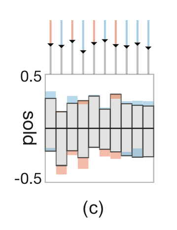
Clicking on the glyph for any word highlights the links to its most responsive hidden state clusters. It also shows the response to the word across all hidden units in a plot in the leftmost column (labelled ‘E’ in the figure).
The hidden state cluster are represented by the ‘memory chip’ visualisations as seen in column C.
We visualize each hidden state unit as a small square-shaped memory cell and pack memory cells in the same cluster into a rectangular memory chip to allow exploration of details.
Within the memory chip, the blue/orange colour coding is once again used to represent the response value of the hidden state units when input words are selected.
Word clusters are naturally visualised as word clouds (column D). The connections between hidden state clusters and word clusters are shown as connecting lines between the corresponding memory chip and word cloud. Blue and orange are used to encode positive/negative contributions, and the width of the connecting line represents the strength of the correlation.
It is possible to interactively select two or three words in the word clouds and compare the model’s responses to these words in an overlay manner. The response of hidden state vectors across several words can also be compared. You can also do a very neat side-by-side comparison of two different models to understand their behaviour on the same inputs:

(Enlarge)
Case studies
Two case studies are highlighted in section 7. The first explores the comparative behaviour of a vanilla RNN, a GRU, and three different LSTMs on a language modelling task. The second case study analyses a sentiment analysis GRU trained on the Yelp Data Challenge dataset. Here for example the co-clustering visualisation clearly showed two different word clouds for words with positive and negative sentiments.
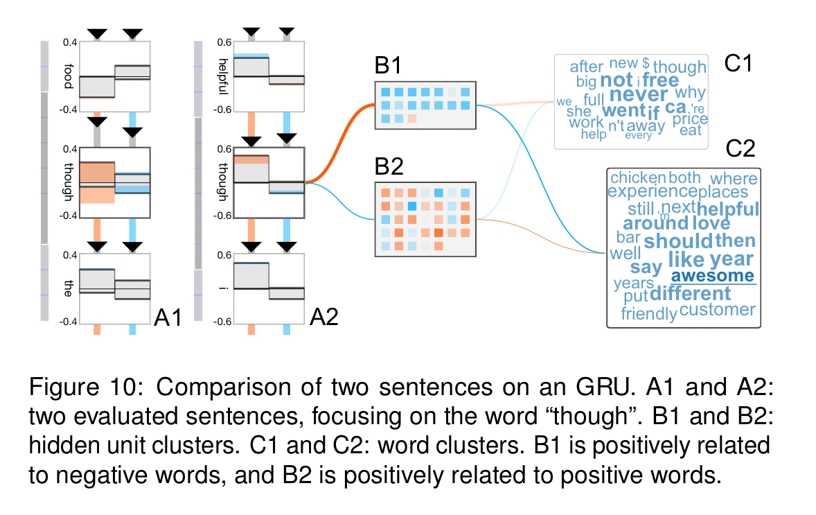
Also of interest in that figure is that the visualisation revealed the GRU had learned to distinguish differing impacts of the word ‘though’ based on context: the response to ‘though’ in ‘I love the food, though the staff is not helpful,’ and ‘The staff is not helpful, though I love the food’ is different in each case (more impactful in the former).
To further improve our proposed visual analytic system, RNNVis, we plan to deploy it online, and improve the usability by adding more quantitative measurements of RNN models… A current bottleneck for RNNvis is the efficiency and quality of co-clustering, which may result in delays during interaction. Other potential future work includes the extension of our system to support the visualization of specialized RNN-based models, such as memory networks or attention models.