The tradeoffs of large scale learning Bottou & Bousquet, NIPS’07
Welcome to another year of The Morning Paper. As usual we’ll be looking at a broad cross-section of computer science research (I have over 40 conferences/workshops on my list to keep an eye on as a start!). I’ve no idea yet what papers we’ll stumble across, but if previous years are anything to go by I’m sure there’ll be plenty of great material to keep interest levels high.
To start us off, today’s paper choice is “The tradeoffs of large scale learning,” which won the ‘test of time’ award at NeurIPS last month.
this seminal work investigated the interplay between data and computation in ML, showing that if one is limited by computing power but can make use of a large dataset, it is more efficient to perform a small amount of computation on many individual training examples rather than to perform extensive computation on a subset of the data. [Google AI blog: The NeurIPS 2018 Test of Time Award].
For a given time/computation budget, are we better off performing a computationally cheaper (e.g., approximate) computation over lots of data, or a more accurate computation over less data? In order to get a handle on this question, we need some model to help us think about how good a given solution is.
Evaluating learning systems
Consider an input domain 

 \in \mathcal{X} \times \mathcal{Y}")
")
")


")

")
The ‘gold standard’ function 
")

")
When we build a given learning model, we constrain the set of prediction functions that can be learned to come from some family 

The optimal function 
We also have an estimation error 
 - E(f^*_{\mathcal{F}})")
The estimation error is determined by the number of training examples and by the capacity of the family of functions. Large families of functions have smaller approximation errors but lead to higher estimation errors.
Now, given that we’re working from training samples, it should be clear that the the empirical risk 


So now we have a trade-off involving three variables and two constraints:
The constraints are the maximal number of available training examples and the maximal computation time. The variables are the size of the family of functions
.
Typically the error components change with respect to the variables as shown in the following table:
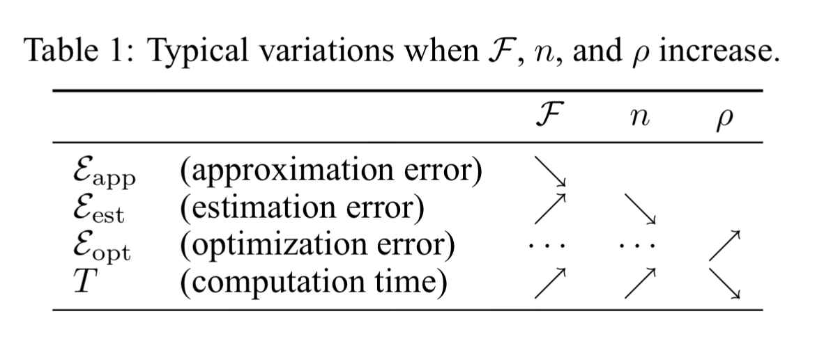
When we are constrained by the number of available training examples (and not by computation time) we have a small-scale learning problem. When the constraint is the available computation time, we have a large-scale learning problem. Here approximate optimisation can possibly achieve better generalisation because more training examples can be processed during the allowed time.
Exploring the trade-offs in large-scale learning
Armed with this model of learning systems, we can now explore trade-offs in the case of large-scale learning. I.e., if we are compute bound, should we use a coarser-grained approximation over more data, or vice-versa? Let’s assume that we’re considering a fixed family of functions
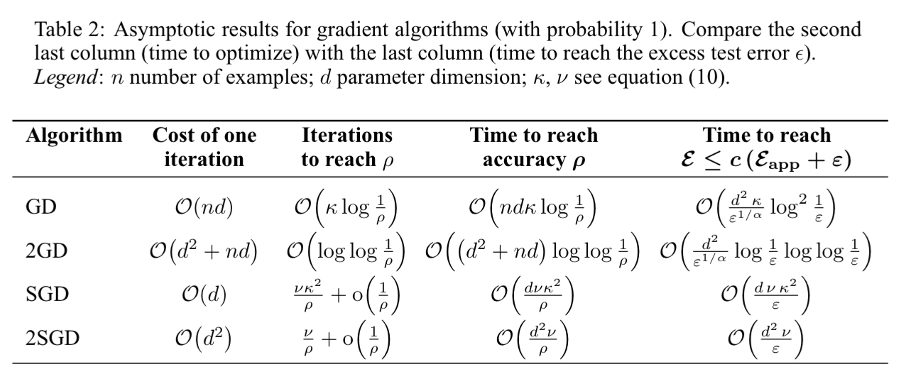
Four gradient descent algorithms are compared:
- Gradient descent, which has linear convergence and requires
iterations to reach accuracy
- Second order gradient descent (2GD), which requires
iterations to reach accuracy
- Stochastic gradient descent, in which a random training example is chosen at each iteration, and the parameters are updated on the basis of that example only. It reaches accuracy
iterations on average. Neither the initial value of the parameter vector nor the total number of examples appear in the dominant term of the bound.
- Second order stochastic gradient descent, which doesn’t change the influence of
The results are summarised in the following table. The third column, time to reach a given accuracy, is simply the cost per iteration (column one) times the number of iterations needed (column two). The fourth column bounds the time needed to reduce the excess error below some chosen threshold.
Setting the fourth column expression to
and solving for
yields the best excess error achieved by each algorithm within the limited time
- SGD and 2SGD results do not depend on the estimation rate exponent,
. When the estimate rate is poor, there is less need to optimise accurately and so we can process more examples.
- Second order algorithms bring little asymptotic improvements, but do bring improvements in the constant terms which can matter in practice.
- Stochastic algorithms yield the best generalization performance despite being the worst optimization algorithms.
The perspective proposed by Léon and Olivier in their collaboration 10 years ago provided a significant boost to the development of the algorithm that is nowadays the workhorse of ML systems that benefit our lives daily, and we offer our sincere congratulations to both authors on this well-deserved award. [Google AI blog: The NeurIPS 2018 Test of Time Award].