Learning the structure of generative models without labeled data Bach et al., ICML’17
For the last couple of posts we’ve been looking at Snorkel and BabbleLabble which both depend on data programming – the ability to intelligently combine the outputs of a set of labelling functions. The core of data programming is developed in two papers, ‘Data programming: creating large training sets, quickly’ (Ratner 2016) and today’s paper choice, ‘Learning the structure of generative models without labeled data’ (Bach 2017).
The original data programming paper works explicitly with input pairs (x,y) (e.g. the chemical and disease word pairs we saw from the disease task in Snorkel) which (for me at least) confuses the presentation a little compared to the latter ICML paper which just assumes inputs 
A generative probabilistic model for accuracy estimation under independence
We have input data points 


Each labelling functions takes as input an data point 


We start out by assuming that the outputs of the labelling functions are conditionally independent given the true label. Consider a labelling function 


 = y_i \Lambda_{ij}")
The accuracy function itself is controlled by some parameter 
Now for 
where 

The unknown parameters 
We can do this using standard stochastic gradient descent, where the gradient for parameter 
Structure learning
The conditionally independent model is a common assumption, and using a more sophisticated generative model currently requires users to specify its structure.
As we know from the Snorkel paper, unfortunately labelling functions are often not independent.
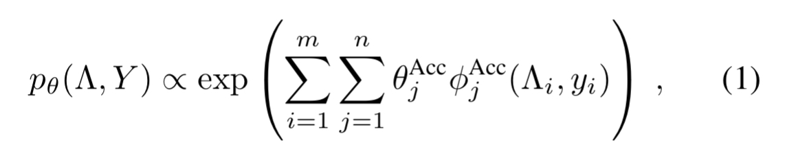
To address this issue, we generalize the conditionally independent model as a factor graph with additional dependencies, including higher-order factors that connect multiple labeling function outputs for each data point
Suppose there is a set 


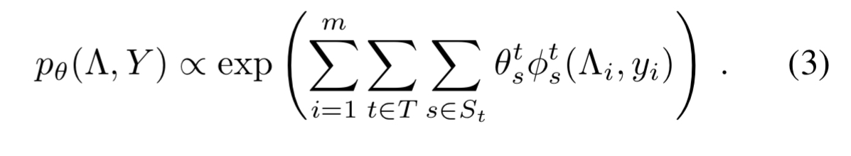
and we want to learn the parameters 
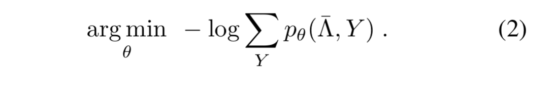
Estimating the structure of the distribution
is challenging because Y is latent; we never observe its value, even during training. We must therefore work with the marginal likelihood
. Learning the parameters of the generative model requires Gibbs sampling to estimate gradients. As the number of possible dependencies increases at least quadratically in the number of labeling functions, this heavyweight approach to learning does not scale.
The way out is to consider each labelling function in turn, optimising the log marginal pseudolikelihood of its outputs conditioned on the outputs of all the other labelling functions.
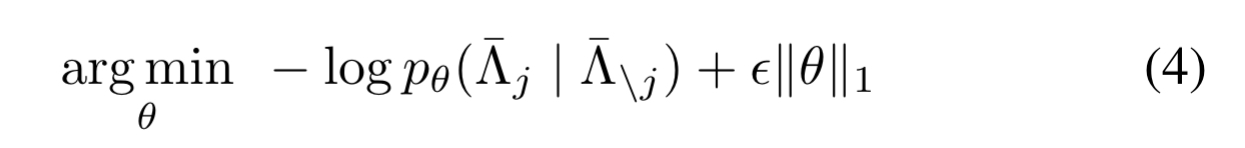
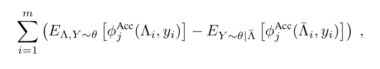
where 
By conditioning on all other labeling functions in each term…, we ensue that the gradient can be computed in polynomial time with respect to the number of labeling functions, data points, and possible dependencies; without requiring any sampling or variational approximations.
It all comes together in the following algorithm:
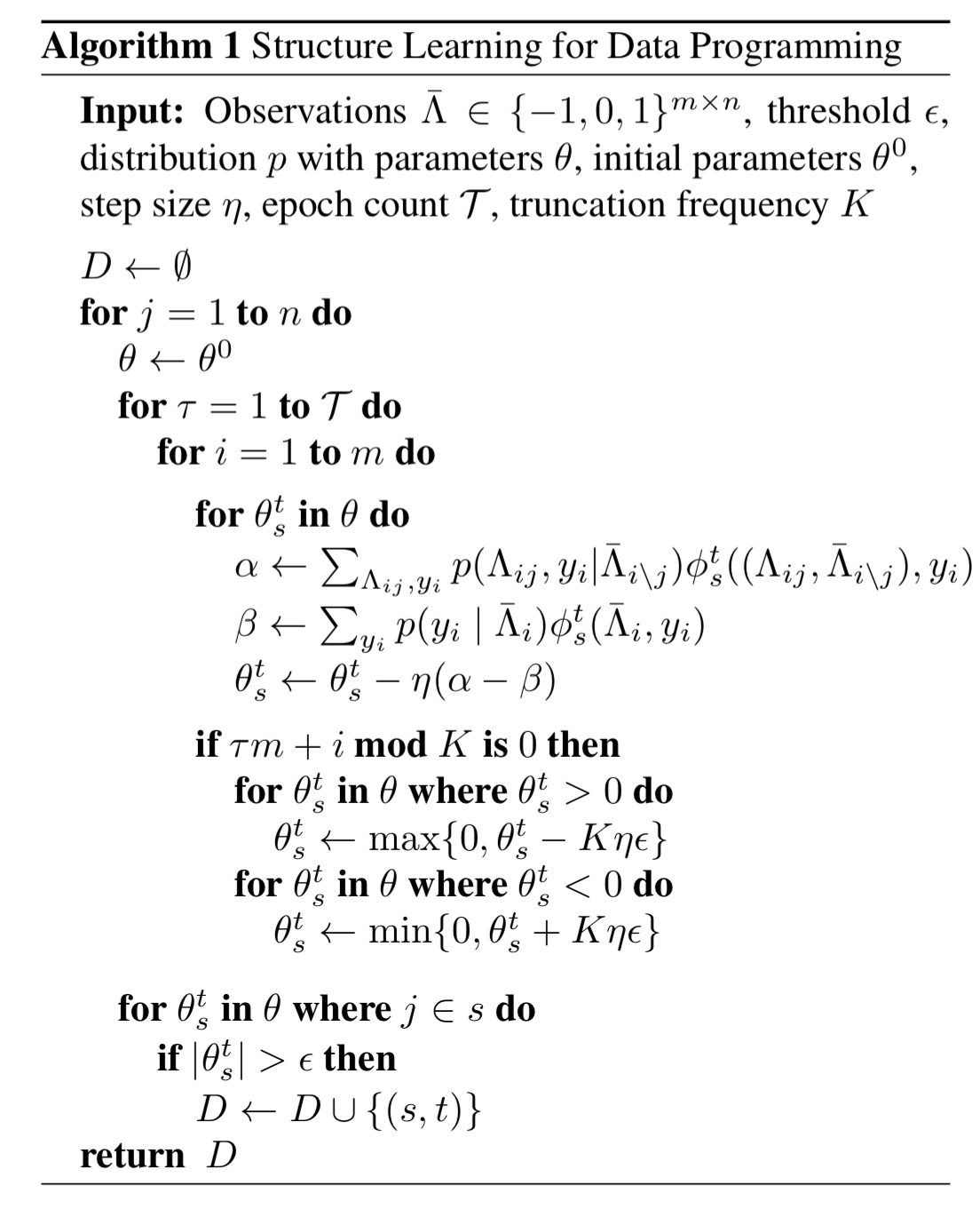
The hyperparameter 
Theoretical guarantees
Assuming that there exist some set of parameters which can capture the true dependencies within the model we are using, and that all non-zero parameters are bounded away from zero (have at least a minimum magnitude 

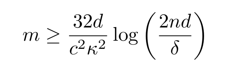
Where 

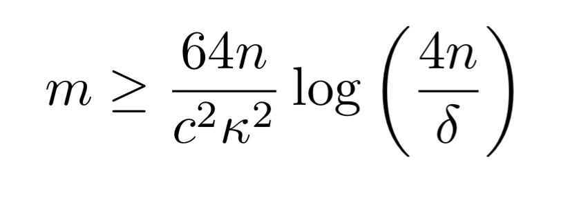
If we further assume that the only dependency types are accuracy and correlation dependencies then we need an input dataset of size
Practical results
Our analysis… guarantees that the sample complexity grows at worst on the order
for
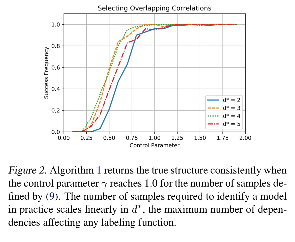
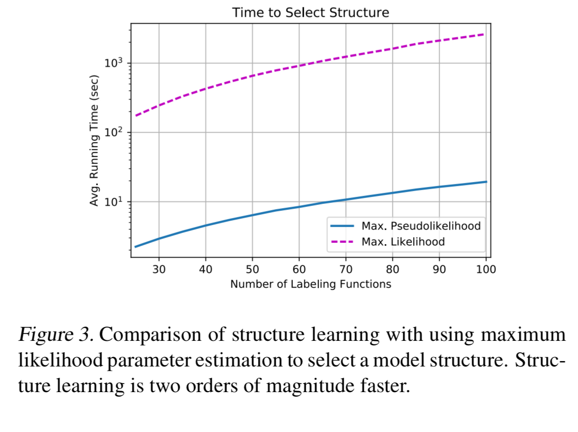
Compared to estimating structures via parameter learning over all possible dependencies, algorithm one is 100x faster and selects only 1/4 of the extraneous correlations.