Progressive growing of GANs for improved quality, stability, and variation Karras et al., ICLR’18
Let’s play “spot the celebrity”! (Not your usual #themorningpaper fodder I know, but bear with me…)
In each row, one of these is a photo of a real person, the other image is entirely created by a GAN. But which is which?
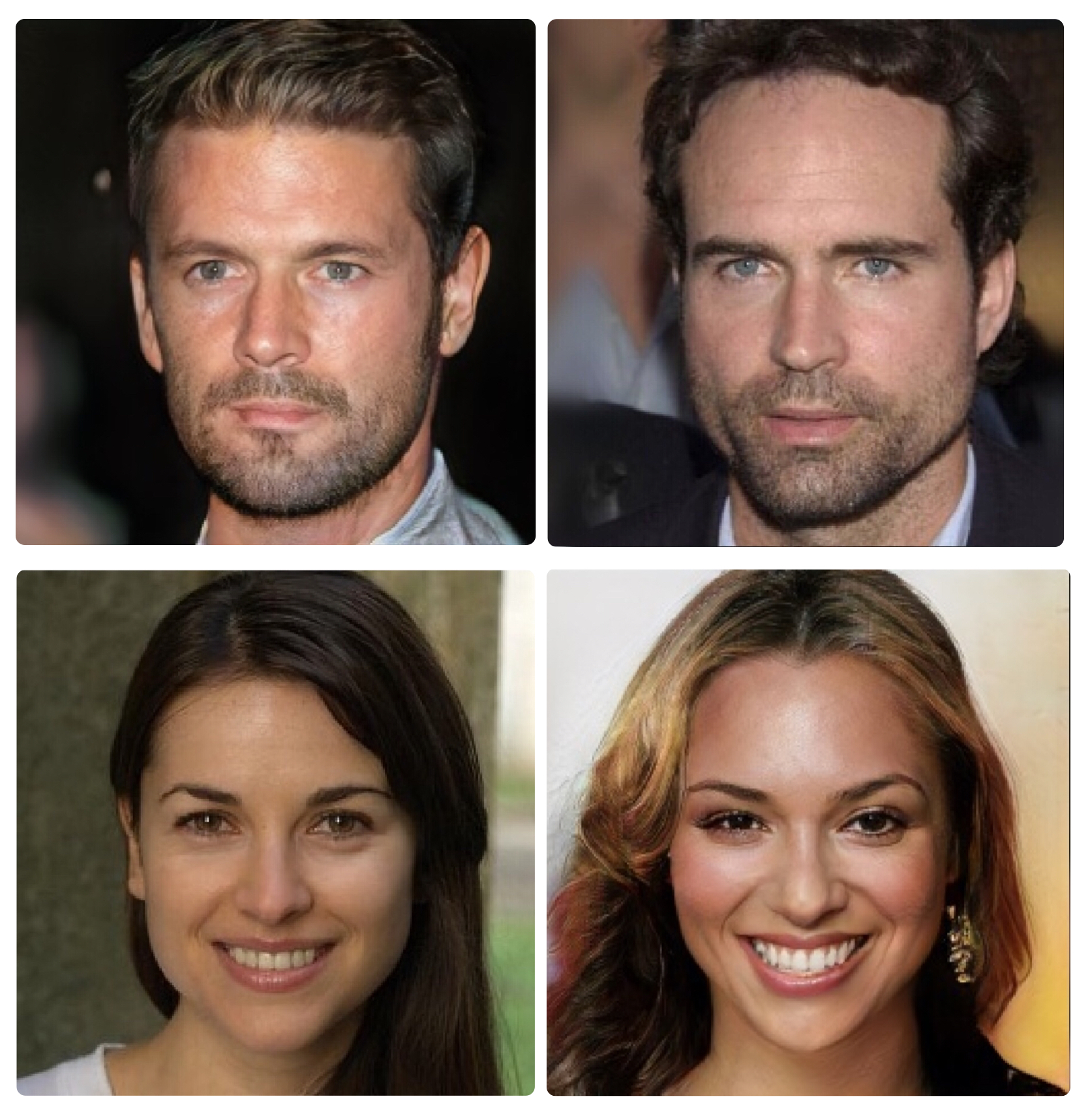
The man on the left, and the woman on the right, are both figments of a computer’s imagination.
In today’s paper, Karras et al. demonstrate a technique for producing high-resolution (e.g. 1024×1024) realistic looking images using GANs:
The key idea is to grow both the generator and discriminator progressively: starting from a low resolution, we add new layers that model increasingly fine details as training progresses. This both speeds the training up and greatly stabilizes it, allowing us to produce images of unprecedented quality.
You can find all of the code, links to plenty of generated images, and videos of image interpolation here: https://github.com/tkarras/progressive_growing_of_gans. This six-minute results video really showcases the work in a way that it’s hard to describe without seeing. Well worth the time if this topic interests you.
[youtube https://youtu.be/G06dEcZ-QTg]
Progression
Recall that in a GAN setup we pitch a generator network against a discriminator network, using the differentiable discriminator as an adaptive loss function. A problem arises (‘the gradient problem’) when the generated and training images are too easy to tell apart.
When we measure the distance between the training distribution and the generated distribution, the gradients can point to more or less random directions if the distributions do not have substantial overlap…
With higher resolution images, it becomes easier to spot the generated images from the real thing, making the gradient problem much worse. It’s asking a lot of the generator network to master everything from large scale structure to fine detail in one hit.
Kerras et al. have a clever solution. They start with small (always matching in size) generator and discriminator networks trained on low resolution images. Then step by step they add in additional layers, and train with increasingly higher resolution images. Like this:
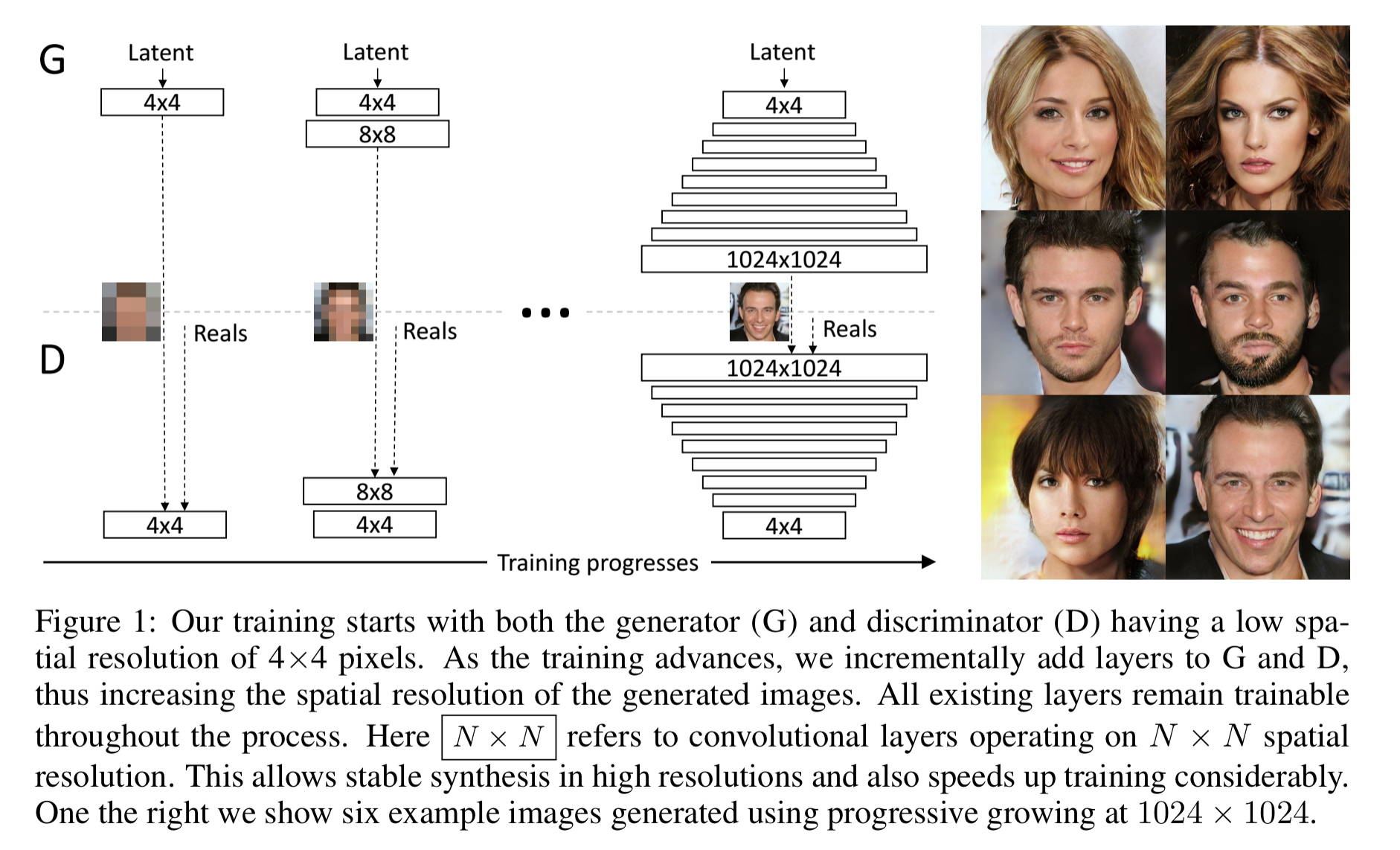
This incremental nature allows the training to first discover large-scale structure of the image distribution, and the shift attention to increasingly finer-scale detail, instead of having to learn all scales simultaneously… All existing layers in both networks remain trainable throughout the training process. When new layers are added to the networks, we fade them in smoothly. This avoids sudden shocks to the already well-trained, smaller-resolution layers.
This progressive training adds stability to the whole process. Early on, small images are easier to generate because there is less class information and fewer modes. When increasing the resolution bit-by-bit we are asking much simpler questions of the network compared to directly discovering a mapping from latent vectors to images of a given size from scratch. The training is sufficiently stabilised to be able to synthesize megapixel-scale images using Wasserstein loss (WGAN-GP), and even least-squares based loss.
You can see the benefits of progressive training in these plots of sliced Wasserstein distance (SWD) between generated and training images, and training time.
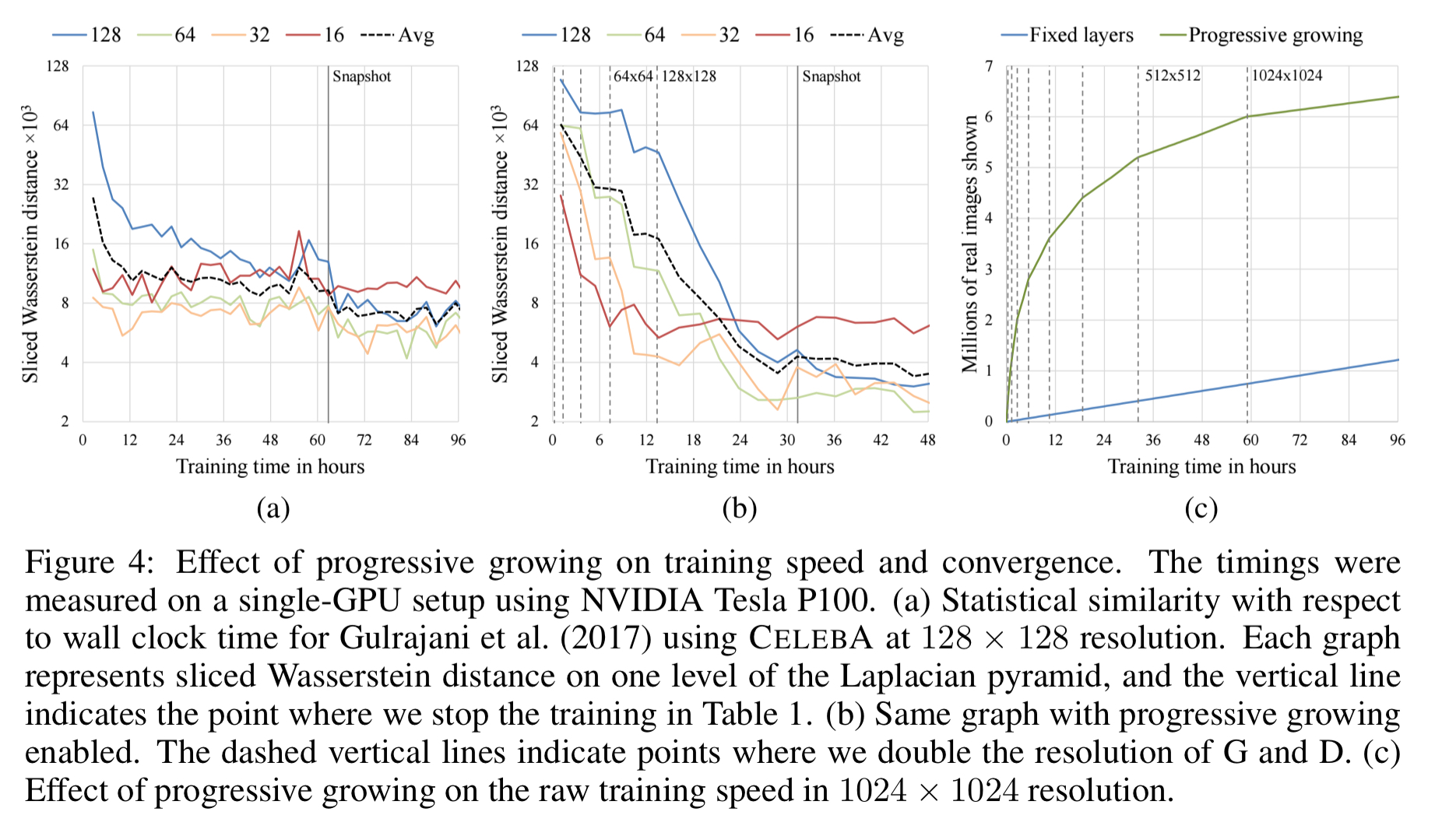
On the left (a) is a standard (non-progressive) GAN. In the middle chart (b), we see the same plot for a progressive GAN. Note the different scales in the x-axis when comparing. You can see the similarity curves level off one-by-one, achieving better accuracy than (a) in much less training time. On the right (c), you see on of the secrets to getting better results in much less time: with smaller images at the start of training, it’s possible to get through a lot more of them. So whereas it takes the non-progressive GAN about 72 hours to process 1 million (full-size) images, the progressive GAN gets there in what looks to be about an hour. The speed advantage of the progressive GAN diminishes later in training as it moves on to bigger images (the point at which the tangent to the green line starts to run parallel with the blue line).
Variation
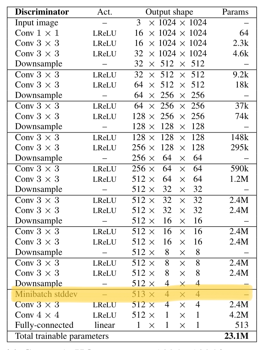
GANs have a tendency to capture only a subset of the variation found in training data, and Salimans et al. suggest “minibatch discrimination” as a solution. They compute feature statistics not only from individual images, but also across the minibatch, thus encouraging the minibatches of generated and training images to show similar statistics.
In this work, Kerras et al. compute the std deviation for each feature in each spatial location over a minibatch, and average over the lot to arrive at a single value. This value is replicated and used to create a constant feature map layer inserted towards the end of the discriminator.
Normalisation
GANs are prone to the escalation of signal magnitudes as a result of unhealthy competition between the two networks. Most if not all earlier solutions discourage this by using a variant of batch normalization… we deviate from the current trend of careful weight initializiation, and instead use a trivial N(0,1) initialization and then explicitly scale the weights at runtime.
The weights in each layer are divided by a per-layer normalisation constant (taken from He’s initialiser). Adaptive stochastic gradient descent methods (e.g. Adam, RMSProp) normalise a gradient update by its estimated standard deviation. If some parameters have a larger dynamic range than others, they will take longer to adjust. Thus a single learning rate can be both too large and too small at the same time. The scaling approach taken here ensure that the dynamic range, and hence the learning speed, is the same for all weights. To prevent escalating competition in feature vector magnitudes, the feature vectors in each pixel are also normalised to unit length in the generator after each convolutional layer.
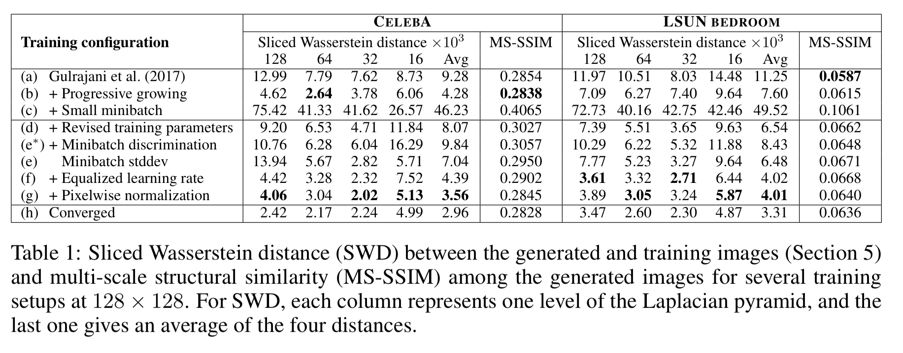
The following table shows the impact of the individual contributions as we build towards the full model:
Experiments
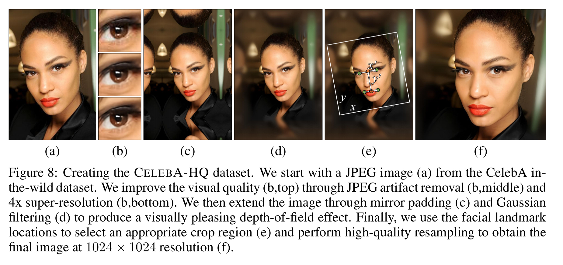
If you carefully study the generated images for the celebrity dataset (CelebA), you’ll see some artifacts such as aliasing, compression, and blur. These aren’t failings of the generator. In fact, they exist in the training images, and the generator has learned to faithfully reproduce them! Since the pre-existing CelebA in-the-wild dataset had very mixed resolution images (from 43×55 all the way up to 6732×8984), it was necessary to create a high-quality version of the dataset before training. This ultimately included 30,000 images at 1024×1024. The process for creating them is illustrated below (note the use of a super-resolution network in step b!).
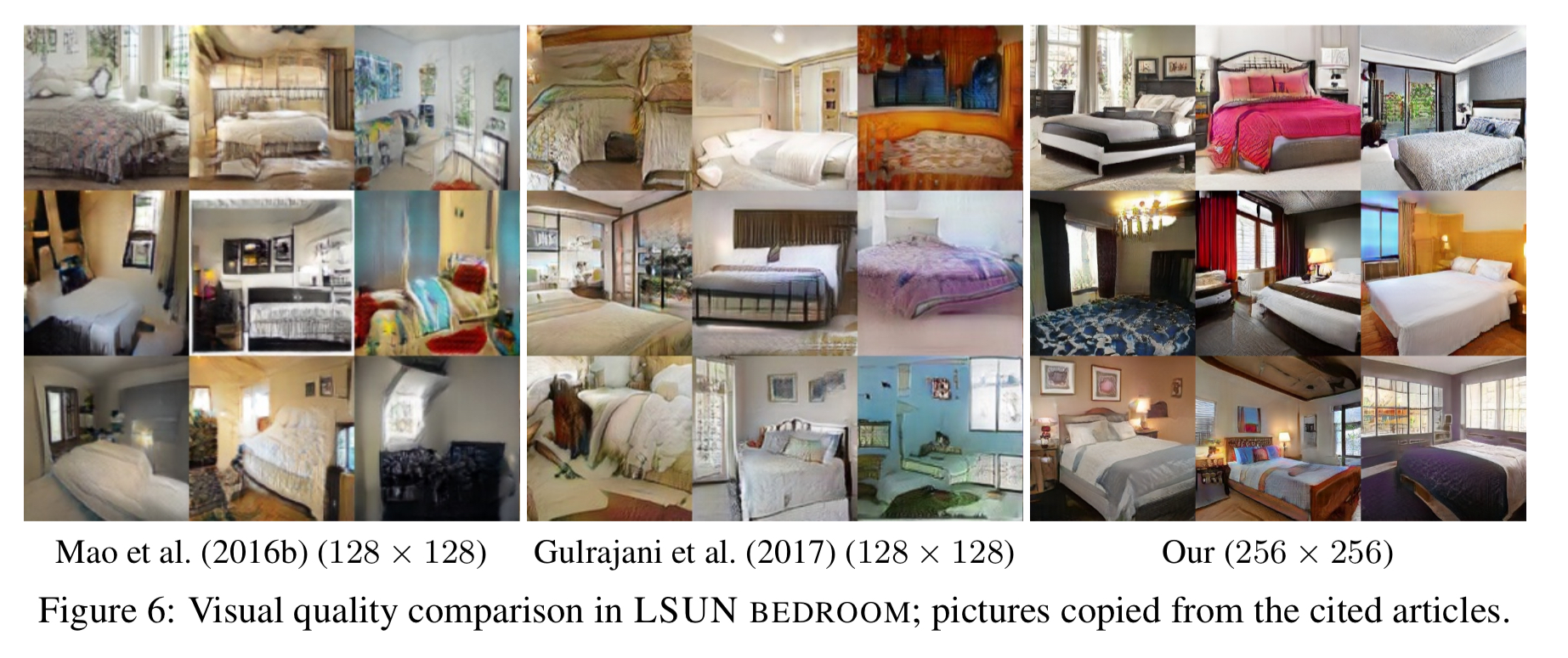
The network can learn any class of image of course, not just faces. Here are some bedroom pictures (rhs), compared against those produced by previous methods:
And here are some generated images for other LSUN categories:
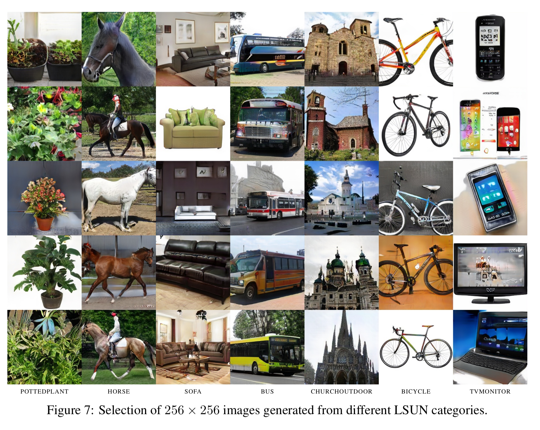
There are loads more in the paper appendix and online.
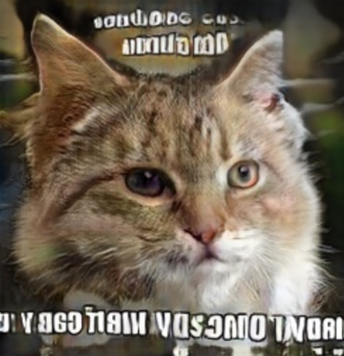
Here I’ve cropped a generated cat image (clearly inspired by Internet meme images), to show where such approaches still struggle. The text is roughly in the right place, but it’s clearly not text we would recognise. Whereas the cat itself looks pretty good!
While the quality of our results is generally high compared to earlier work on GANs and the training is stable in large resolutions, there is a long way to true photorealism. Semantic sensibility and understanding dataset-dependent constraints, such as certain objects being straight rather than curved, leaves a lot to be desired. There is also room for improvement in the micro-structure of the images. That said, we feel that convincing realism may now be within reach, especially in CelabA-HQ.