Performance analysis of cloud applications Ardelean et al., NSDI’18
Today’s choice gives us an insight into how Google measure and analyse the performance of large user-facing services such as Gmail (from which most of the data in the paper is taken). It’s a paper in two halves. The first part of the paper demonstrates through an analysis of traffic and load patterns why the only real way to analyse production performance is using live production systems. The second part of the paper shares two techniques that Google use for doing so: coordinated bursty tracing and vertical context injection.
(Un)predictable load
Let’s start out just by consider Gmail requests explicitly generated by users (called ‘user visible requests,’ or UVRs, in the paper). These are requests generated by mail clients due to clicking on messages, sending messages, and background syncing (e.g., IMAP).
You can see a clear diurnal cycle here, with the highest QPS when both North America and Europe are active in the early morning, and lower QPS at weekends. (All charts are rescaled using some unknown factor, to protect Google information).
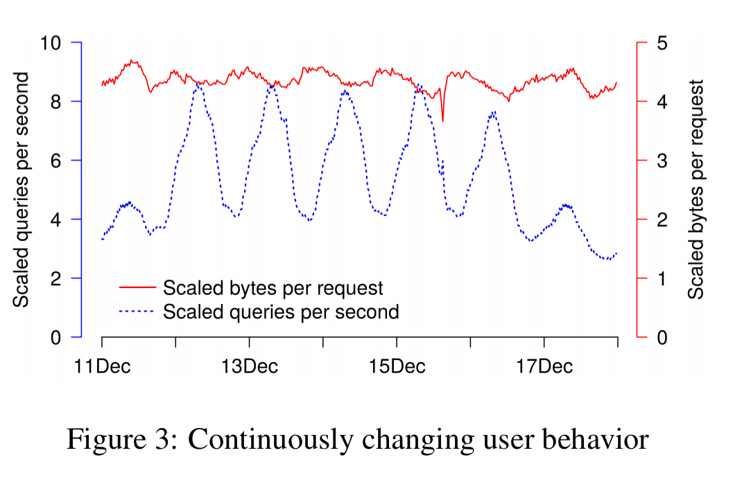
Request response sizes vary by about 20% over time. Two contributing factors are bulk mail senders, sending bursts of email at particular times of the day, and IMAP synchronisation cycles.
In summary, even if we consider only UVR, both the queries per second and mix of requests changes hour to hour and day to day.
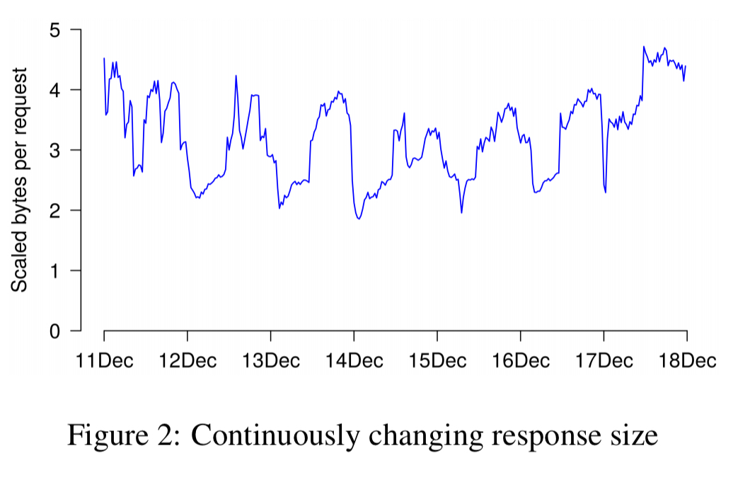
If we look at the total load, we see it’s significantly less predictable than the UVR patterns would lead us to believe.
Drilling into request response size, we see that it varies by a factor of two over the course of the week and from hour to hour. The actual mix of requests to the system (and not just the count of requests) changes continuously.
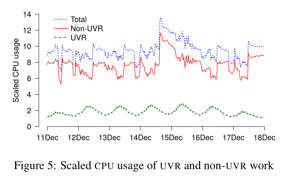
There are multiple reasons for this: system tasks continuously validating data integrity and recovering from failures; the rollout of software updates; repairs due to bugs (e.g., reindexing messages), and underlying data management tasks such as Bigtable compaction. Combining these non-UVR tasks with UVR load in one chart reveals these non-UVR tasks have a significant impact on CPU usage, with UVR work directly consuming only about 20% of CPU.
Then of course, there are the one-off events, such as the time that Google’s Belgian datacenter was struck by lightning four times, potentially corrupting data on some disks. Reconstructing it and rebalancing requests while that went on caused quite a bit of disruption!
Limitations of synthetic workloads
The superimposition of UVR load, non-UVR load, and one-off events results in a complex distribution of latency and resource usage, often with a long tail. When confronted with such long-tail performance puzzles, we first try to reproduce them with synthetic users…
Despite best efforts at modelling though, the synthetic test environment often shows different behaviours to production. It can serve as a general guide though: the relationships uncovered in synthetic testing are often valid, if not the magnitude of the effect. I.e., if an optimization improves latency of an operation with synthetic users it will often also do so for real users, but by a varying amount.
For most subtle changes though, we must run experiments in a live system serving real users.
High level methodology
Users are partitioned (randomly), with one partition as the test and the other as the control. It turns out that we need large samples! Here’s a A/A test chart with two 100K user partitions – we expect them to have identical latency distributions of course. By the 95th percentile latencies differ by up to 50% and often by at least 15%.
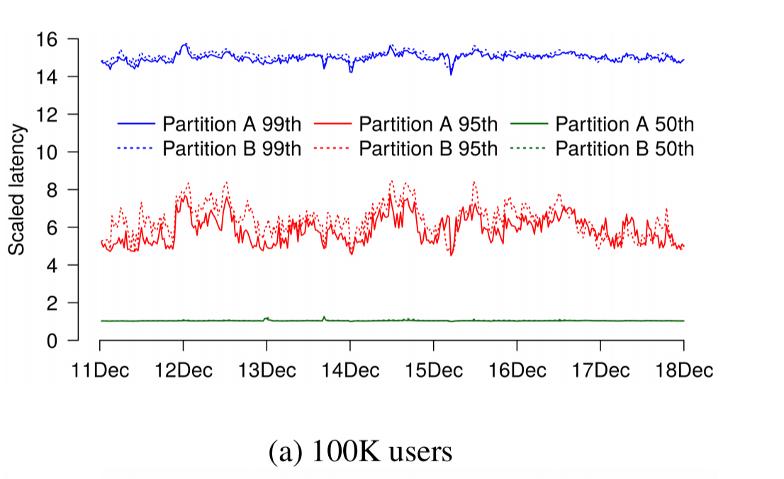
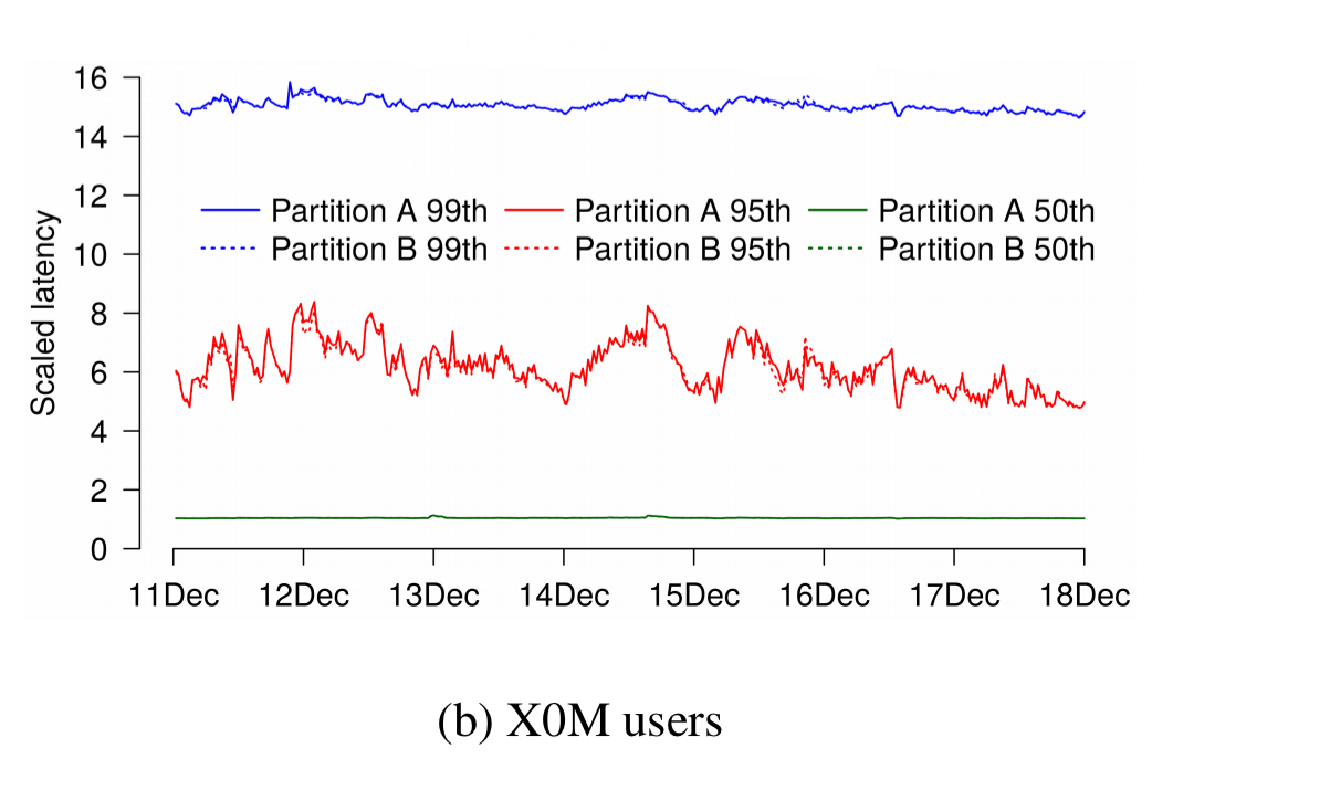
Only in an A/A test with partitions containing tens of millions of users do we find partition results that are largely indistinguishable from each other.
Given that many fields routinely derive statistics from fewer than 100K observations, why do our samples differ by up to 50% at some points in time? The diversity of our user population is responsible for this: Gmail users exhibit a vast spread of activity and mailbox sizes with a long tail.
As a result of this, tests are done in a live application settings with each experiment involving millions of users. Longitudinal studies take place over a week or more to capture varying load mixes. Comparisons between test and control are primarily done at the same points in time. Statistics are used to analyse the data and predict the outcome of risky experiments and to corroborate the results with other data.
Statistics: handle with care
The choice of statistical methods is not always obvious: most methods make assumptions about the data that they analyze (e.g., the distribution or independence of the data)… any time we violate the assumptions of a statistical method, the method may produce misleading results.
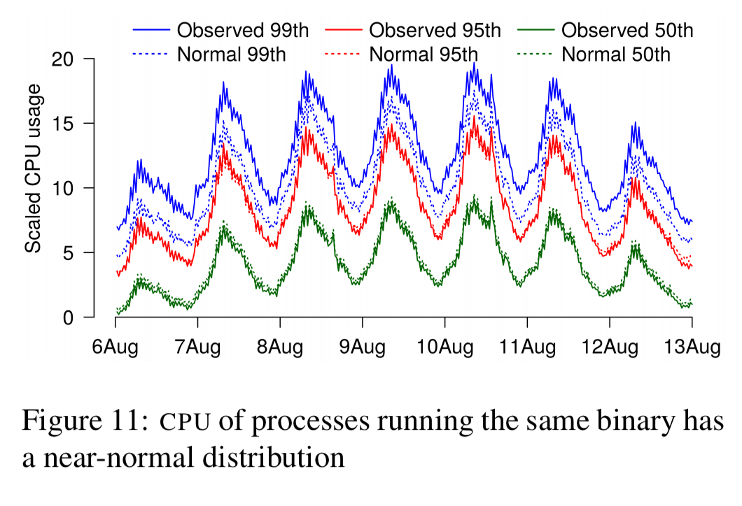
Here’s an example when it worked: modelling the predicted CPU demands when doubling the number of users. The distribution of CPU usage for N processes exhibits a near normal distribution. Thus in theory, the properties of 2N processes could be calculated using the standard methods for adding normal distributions (to add a distribution to itself, double the mean and take the square route of the standard deviation). The predicted CPU usage matched well with actuals (within 2%) at the 50th and 95th percentiles, but underestimate at the 99th. With the exception of this tail, the model worked well.
Another experiment tried to model what would happen when co-locating pairs of communicating processes. This time the predictions are all over the map compared to the results:
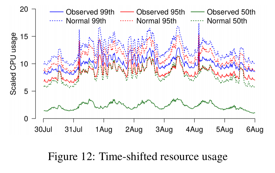
The CPU usage of the two processes is not independent. They exhibit time-shifted CPU usage when the higher-level process makes an RPC call to the lower-level process, and then waits for a response. Because the two distributions are not independent they can’t be added together.
Time and motion
Before we can determine what changes we need for a cloud application to become more responsive or cost effective, we need to understand why a request to a cloud application is slow or expensive. To achieve that understanding we need to consider two contexts…
- The temporal context of a request tells you what else was going on at the time.
- The operation context tells you how a single request flows through many processes and software layers. The operation context helps to tease apart the differences between generally slow calls, calls that are slow with certain arguments, and calls that are individually fast but large numbers of them add up to a slow request.
On your marks, get set, trace…
The obvious approach for using sampling yet getting the temporal context is to use bursty tracing. Rather than collecting a single event at each sample, bursty-tracing collects a burst of events.
We need to capture events across processes / layers at the same point in time for this to work, which requires some kind of coordination so that everyone knows when to stop and start tracing. Google have a very pragmatic approach to this which avoids the need for any central coordination – just use the wall clock time! A burst config determines the on-and-off periods for tracing (e.g. trace for 4ms every 32ms). Bursts last for 2^n ms, with one burst every 2^(n+m) ms. This can be encoded as m 1s followed by n 0s in binary. Each process then performs tracing whenever burst-config & WallTimeMillis() == burst-config, which it can determine entirely locally.
This scheme does require aligned wall clocks across machines, but of course Google have true time for that!
We use coordinated bursty tracing whenever we need to combine traces from different layers to solve a performance mystery.
System call steganography
To get the operation context, we need to track spans within and across processes. “Simply interleaving traces based on timestamps or writing to the same log file is not enough to get a holistic trace.” The simplest way from the perspective of reconstructing traces is to modify the code to propagate an operation context through all layers and tag all events with it. This can be intrusive and require non-trivial logic though.
“I have a cunning plan, my lord.”
Our approach relies on the insight that any layer of the software stack can directly cause kernel-level events by making system calls. By making a stylized sequence of innocuous system calls, any layer can actually inject information into the kernel traces.
For example, to encode ‘start of an RPC’ into a kernel trace we can call syscall(getpid, kStartRpc); syscall(getpid, RpcId);. The kernel traces the arguments passed to gitpid, even though getpid ignores them. Two getpid calls are unlikely to naturally occur like this back to back. If kStartRpc is the code for an RPC start, and RpcId is an identifier for the rpc in question, we can look for this pattern in the kernel trace and recover the information. It took less than 100 lines of code it implement RPC and lock-injection information into kernel traces using this scheme.
We use vertical context injection as a last resort: its strength is that it provides detailed information that frequently enables us to get to the bottom of whatever performance mystery we are chasing; its weakness is that these detailed traces are large and understanding them is complex.
The strategies described in the paper have been used for analyzing and optimizing various large applications at Google including Gmail (more than 1 billion users) and Drive (hundreds of millions of users).