The case for learned index structures Kraska et al., arXiv Dec. 2017
Yesterday we looked at the big idea of using learned models in place of hand-coded algorithms for select components of systems software, focusing on indexing within analytical databases. Today we’ll be taking a closer look at range, point, and existence indexes built using this approach. Even with a CPU-based implementation the results are impressive. For example, with integer datasets:
As can be seen, the learned index dominates the B-Tree index in almost all configurations by being up to 3x faster and being up to an order-of-magnitude smaller.
As we left things yesterday, the naive learned index was 2-3x slower! Let’s take a look at what changed to get these kinds of results.
Learned range indexes
Recall that a single learned CDF has difficulty accurately modelling the fine structure of a data distribution. Replacing just the first two layers of a B-Tree though, is much easier to achieve even with simple models. And once we’re dealing with a narrower portion of the data set, learning the fine structure of that becomes much more tractable. So the overall solution is to layer models in a recursive regression model:
…we build a hierarchy of models, where at each stage the model takes the key as an input and based on it picks another model, until the final stage predicts the position.
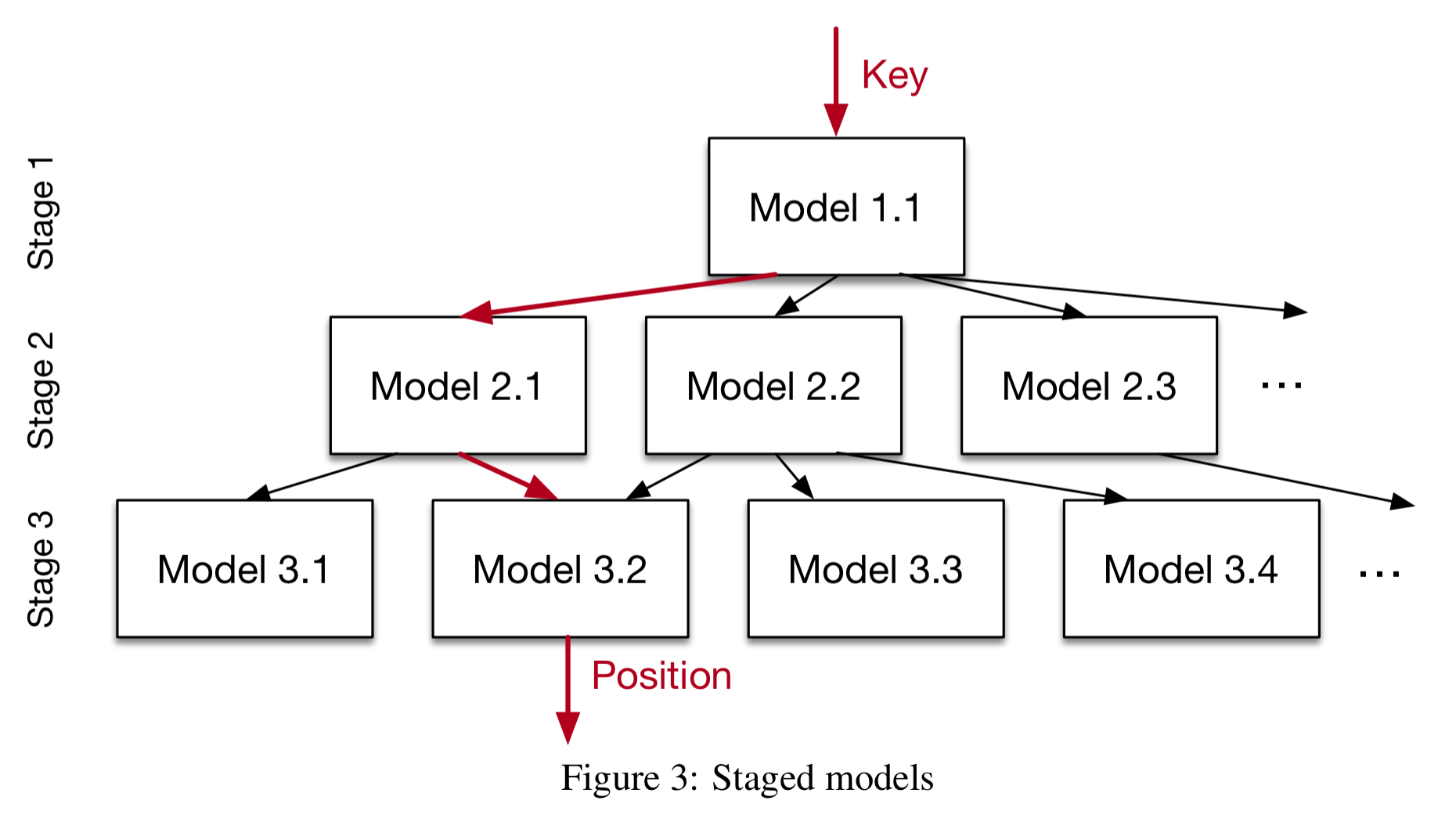
The recursive models are not trees though – different models at the same stage may map to the same models at the next stage. Nor do the models necessarily uniformly divide the key space. Think of model selection more like ‘picking an expert with better knowledge about certain keys.’
Note that we also have the freedom to use different models in the different stages:
For example, whereas on the top-layer a small ReLU neural net might be the best choice as they are usually able to learn a wide-range of complex data distributions, the models at the bottom of the hierarchy might be thousands of simple linear regression models as they are inexpensive in space and execution time.
The entire index (all stages) can be represented as a sparse matrix multiplication for a TPU/GPU, and can be trained end-to-end (see algorithm 1 in §3.3 of the paper).
The output of this Recursive Model Index (RMI) is a page. In absence of any knowledge of the data distribution, traditionally either binary search or scanning (for small page sizes) have been shown to be the fastest strategies. But hold on…
Yet again, learned indexes might have an advantage here as well: the models actually predict the position of the key, which likely to be much closer to the actual position of the record, while the min- and max-error is presumably larger.
Based on this insight, the authors develop a new biased quaternary search strategy. In a quaternary search, instead of picking one new middle point to to test as in binary search, three new test points are chosen (thus dividing the dataset into four quarters, as opposed to two halves). The three initial middle points for the quaternary search are set to be 


For evaluation purposes 4 secondary indexes are created over 3 real-world datasets (with up to 200M rows) and one synthetic dataset designed to exercise heavy-tailed distributions. For all datasets a comparison is done between a very competitive B-Tree implementation, using a variety of page sizes, and 2-stage RMI models with varied second-stage sizes (10K, 50K, 100K, and 200K). Training a full RMI model takes just a few seconds.
Let’s look at the map, weblog, and synthetic log-normal dataset results first, since these all use integer keys.
For the maps dataset, an index is created for the longitude of approximately 200M map features (roads, museums, coffee shops, …). Here’s how the B-Tree and RMI models faired, with total lookup time broken down into model execution time (to find the page) and search time within the page. Results are normalised compared to a B-Tree using 128 page size.
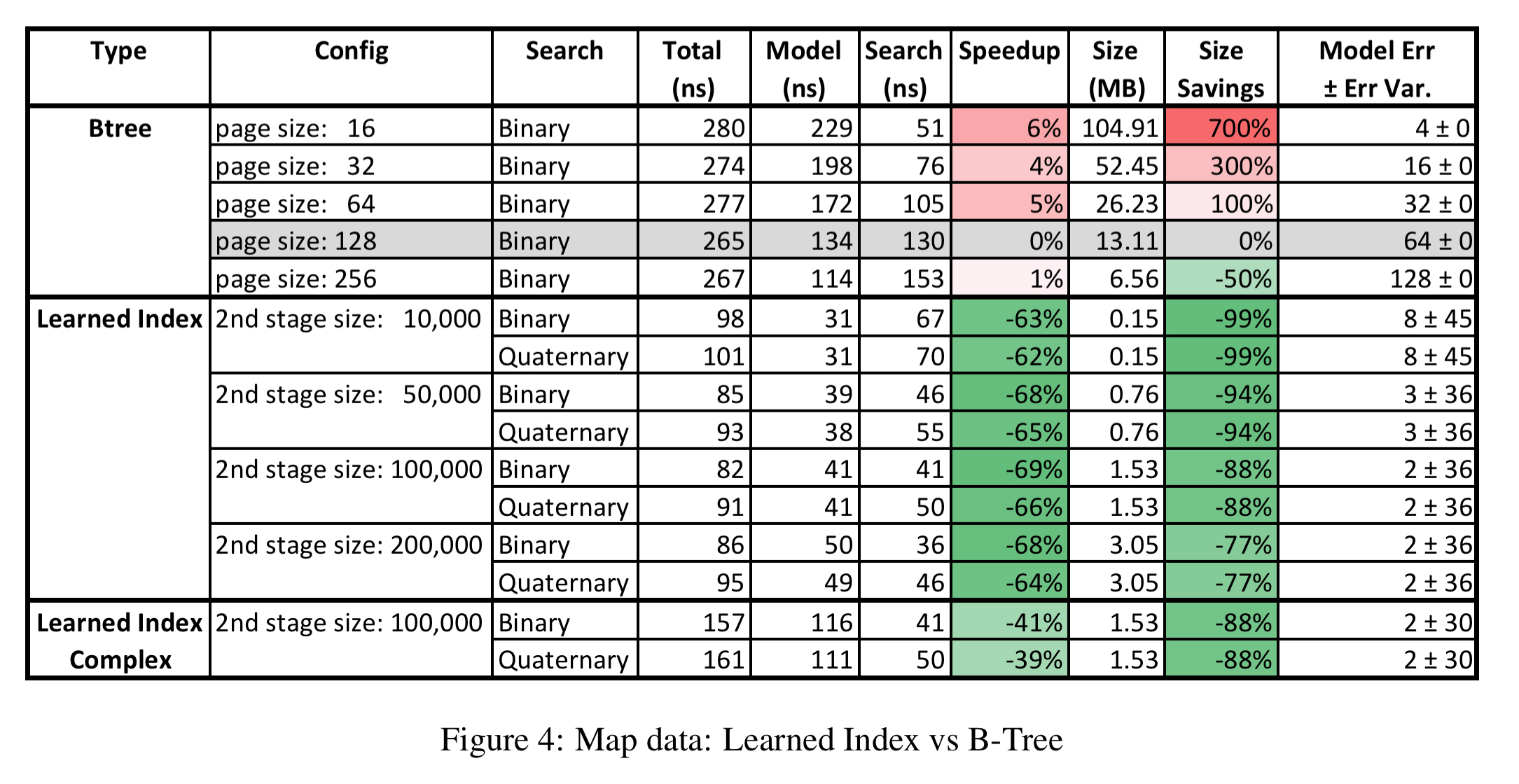
The learned index dominates the B-Tree index: it is up to three times faster and uses significantly less space.
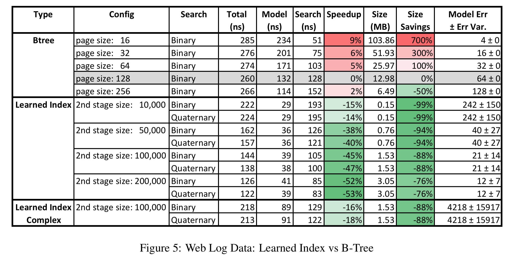
The weblog dataset contains every request to a major university website over several years, and is indexed by timestamp. This is a challenging dataset for the learned model, and yet the learned index still dominates the B-Tree.
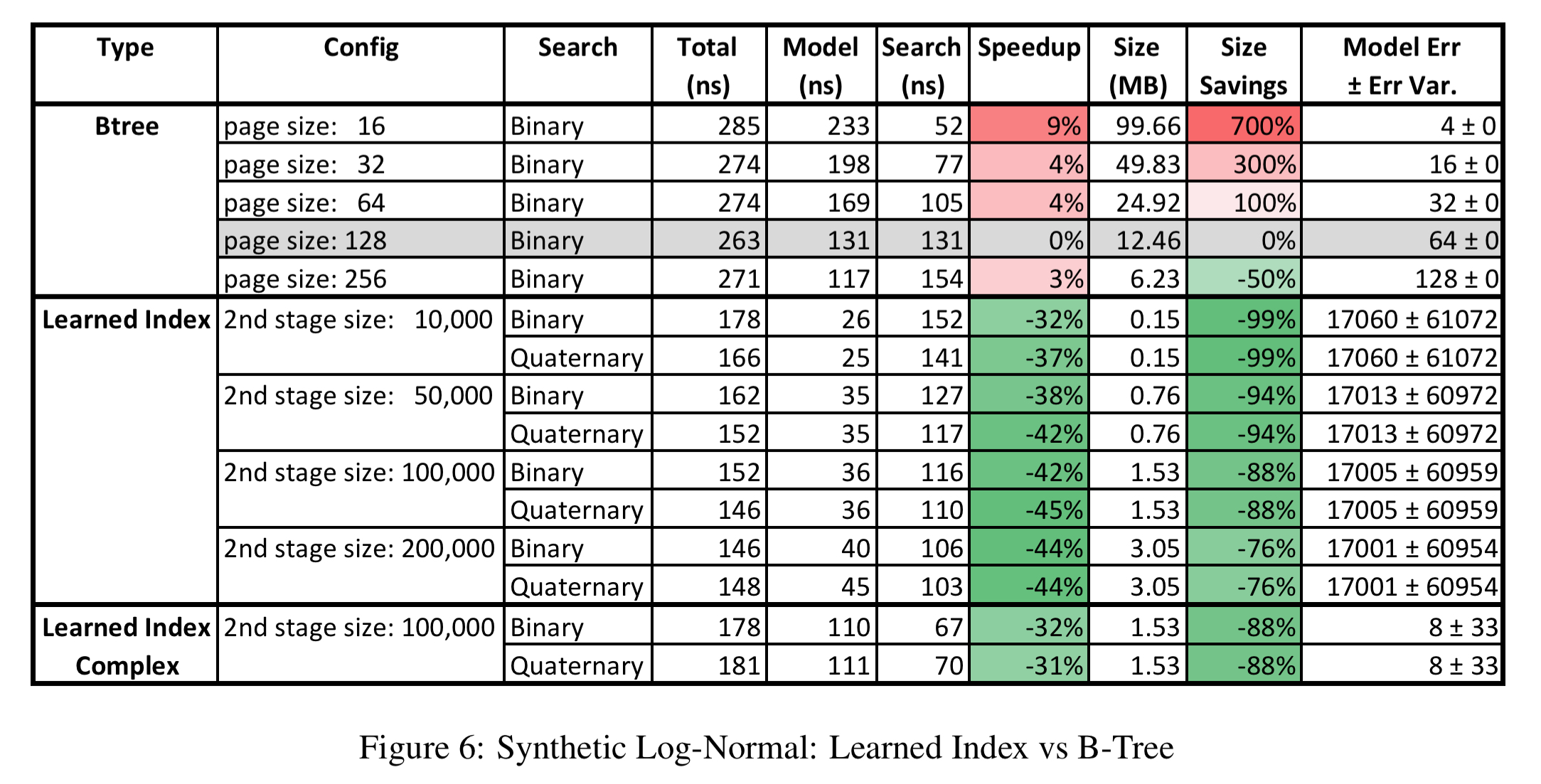
The story is similar with the synthetic log-normal dataset.
The web-documents dataset contains 10M non-continuous document-ids of a large web index. The keys here are strings, and the approach is to turn each string into a max-input length vector with one element per character. Other more sophisticated encodings could be used in the future, exploiting the ability of e.g. RNNs to learn interactions between characters. A hybrid model is included in this set of results, that replaces 2nd-stage models with errors above a threshold with a local B-Tree.
Here the learned index is less obviously better (though it always gives good space savings). Model execution with the vector input is more expensive – a problem that using a GPU/TPU rather than a CPU would solve.
The current design, even without any signification modifications, is already useful to replace index structures as used in data warehouses, which might only be updated once a day, or BigTable where B-Trees are created in bulk as part of the SStable merge process.
It’s possible that learned models have an advantage for certain types of update workloads too – especially if the updates follow the existing data distribution. If the distribution does change, one option is to build a delta-index of inserts and periodically merge it with the main index, including a potential retraining.
Learned point indexes
The key challenge for hash maps is preventing too many distinct keys from mapping to the same position inside the map (a conflict). With e.g., 100M records and 100M slots, there’s roughly a 33% chance of conflict. At this point, we have to use a secondary strategy (e.g., scanning a linked list) to search with the slot.
Therefore, most solutions often allocate significantly more memory (i.e., slots) than records to store… For example, it is reported that Google’s Dense-hashmap has a typical overhead of about 78% of memory.
But if we could learn a model which uniquely maps every key into a unique position inside the array we could avoid conflicts. If you have plenty of memory available, it’s going to be hard to beat the performance of traditional hashmaps. But at higher occupancy rates (e.g., less than 20% overhead) performance starts to slow down significantly and learned models may be able to do better.
Surprisingly, learning the CDF of the key distribution is one potential way to learn a better hash function… we can scale the CDF by the targeted size M of the hash-map and us
, with key K as our hash-function. If the model F perfectly learned the CDF, no conflicts would exist.
This strategy can be used to replace the hash function in any existing hash-map implementation. Here’s an evaluation comparing two-stage RMI models with 100K models in the second stage, against a fast hash function using 3 bitshifts, 3 XORs, and 2 multiplications. For each dataset, the two approaches are evaluated with the number of available slots in the map able to fit from 75% to 125% of the data.
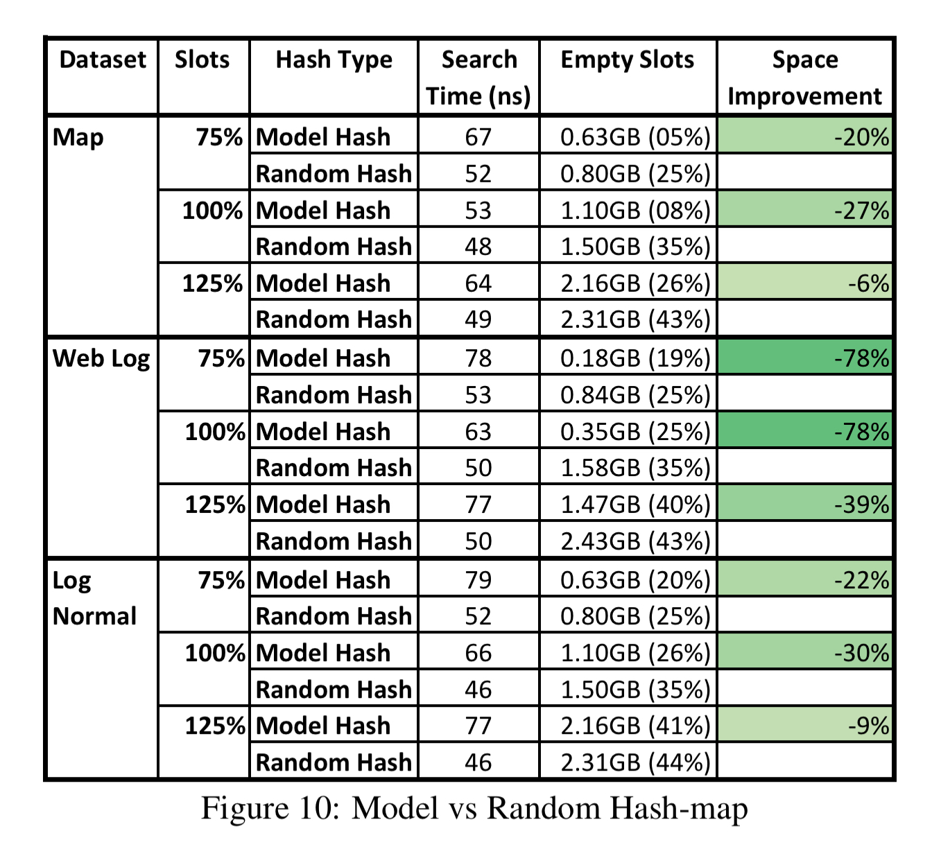
The index with the model hash function overall has similar performance while utilizing the memory better.
Learned existence indexes
Bloom-filters are used to test whether an element is a member of a set, and are commonly used to determine if for example a key exists on cold storage. Bloom filters guarantee that there are no false negatives (if a Bloom filter says the key is not there, then it isn’t there), but do have potential for false positives. Bloom filters are highly space efficient, but can still occupy quite a bit of memory. For 100M records with a target false positive rate of 0.1%, we need about 14x more bits than records. And once more…
… if there is some structure to determine what is inside versus outside the set, which can be learned, it might be possible to construct more efficient representations.
From an ML perspective, we can think of a Bloom-filter as a classifier, which outputs the probability that a given key is in the database. We can set the probability threshold 

The approach was tested using a dataset of 1.7M unique blacklisted phishing URLs together with a negative set of valid URLs. A character-level RNN (GRU) is trained as the classifier to predict which set a URL belongs to. Compared to a normal Bloom filter, the model + spillover Bloom filter gives a 47% reduction in size for the same false positive rate (1%). At 0.01%, the space reduction is 28%.
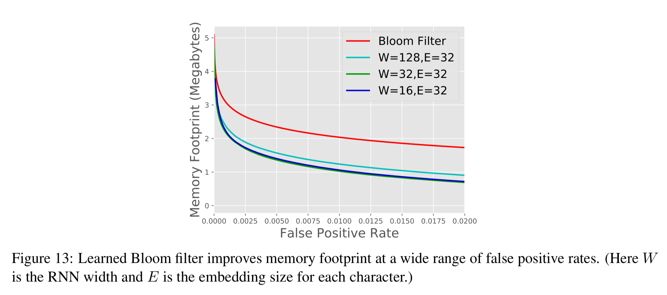
The more accurate the model, the better the savings in Bloom filter size. There’s nothing stopping the model using additional features to improve accuracy, such as WHOIS data or IP information.
The last word
…we have demonstrated that machine learned models have the potential to provide significant benefits over state-of-the-art database indexes, and we believe this is a fruitful direction for future research.
I look forward to seeing more work along on this line!