Continuous online sequence learning with an unsupervised neural network model Cui et al., Neural Computation, 2016
Yesterday we looked at the biological inspirations for the Hierarchical Temporal Memory (HTM) neural network model. Today’s paper demonstrates more of the inner workings, and shows how well HTM networks perform on online sequence learning tasks as compared to other approaches (e.g., LSTM-based networks).
The HTM model achieves comparable accuracy to other state-of-the-art algorithms. The model also exhibits properties that are critical for sequence learning, including continuous online learning, the ability to handle multiple predictions and branching sequences with high-order statistics, robustness to sensor noise and fault tolerance, and good performance without task-specific hyperparameter tuning.
The HTM sequence memory model
Recall from yesterday that the HTM sequence memory model is organised around layers of mini-columns of cells.
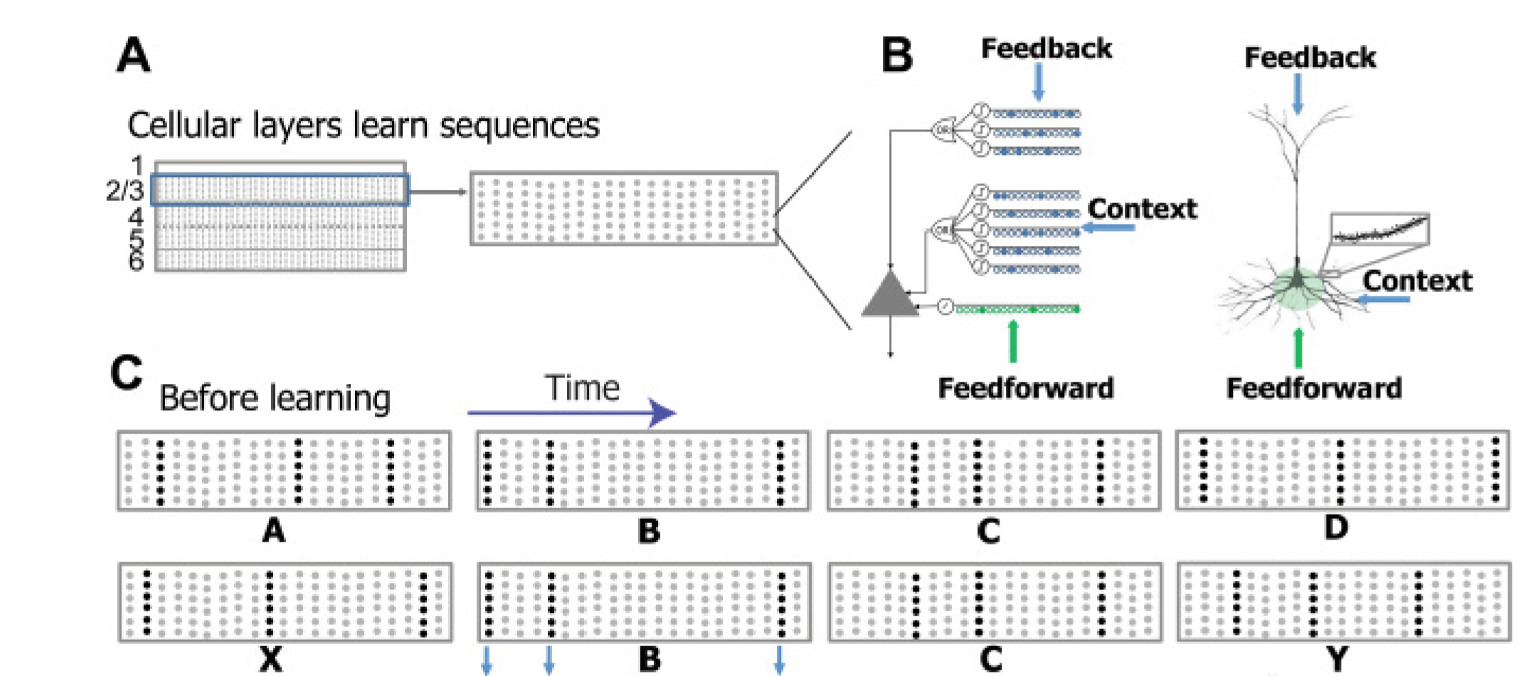
The network represents higher-order (dependent on previous time steps) sequences using a composition of two separate sparse representations. At the column level, each input element is encoded as a sparse distributed activation of columns: the top 2% of columns that receive the most active feedforward inputs are activated. Within an active column, a subset of the cells will be active – if a column contains predicted cells then only these cells will be active, otherwise all cells within the column become active.
A network has 


- The
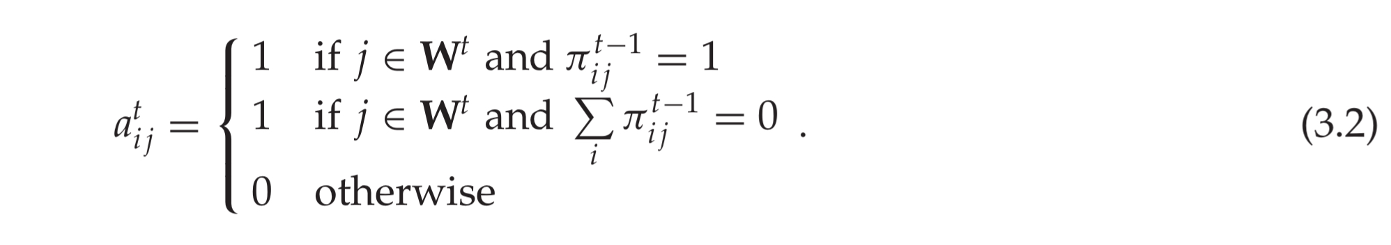
binary matrix
represents the activation state (on/off) of the cells:
is the activation state of the
th cell in the
th column.
- The
represents the predictive state (on/off) of the cells:
is the predictive state of the
Each cell has 


At time step
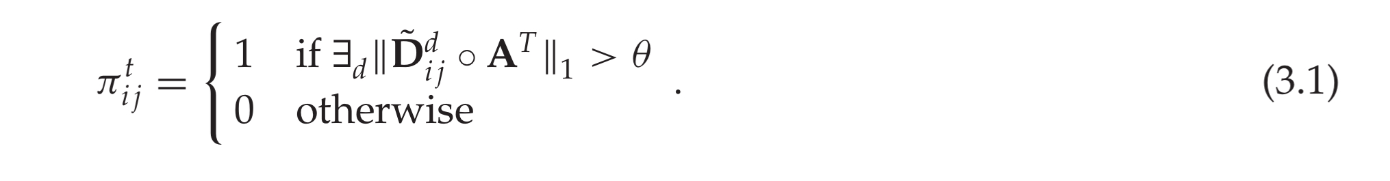
Threshold 

At each time 
A cell is considered active if its column is active and it was in predictive state during the previous time step, or its column is active and none of the other cells in the same column were in a predictive state:
Learning is local and straight forward:
The lateral connections in the sequence memory model are learned using a Hebbian-like rule. Specifically, if a cell is depolarized and subsequently becomes active, we reinforce the dendritic segment that caused the depolarization. If no cell in ac active column is predicted, we select the cell with the most activated segment and reinforce that segment. Reinforcement of a dendritic segment involves decreasing permanence values of inactive synapses by a small value
and increasing the permanence for active synapses by a larger value
.

Where 

Cell that don’t become active also receive a very small decay.
The sequence memory operates with sparse distributed representations (SDRs). Original data is converted to SDRs using an encoder (in this case, a random encoder for categorical data, and scalar date-time encoders for a taxi data experiment). We can’t use a simple one-hot encoding for categorical data because we also want to able to provide noise inputs drawn from a very large distribution. Decoding from SDRs is done using classifiers.
Real-time streaming data analysis
In this paper HTMs are applied to real-time streaming data pattern matching problems where they have the following desirable characteristics:
- they can learn online in a single pass without requiring a buffered data set
- they can make higher-order predictions across multiple time steps, learning the order (number of previous steps to consider) automatically
- they can make multiple simultaneous predictions in the case of ambiguity
- they are robust to the loss of synapses and neurons (important for hardware implementations)
- they do not require any hyperparameter tuning
Sequence prediction with artificial data
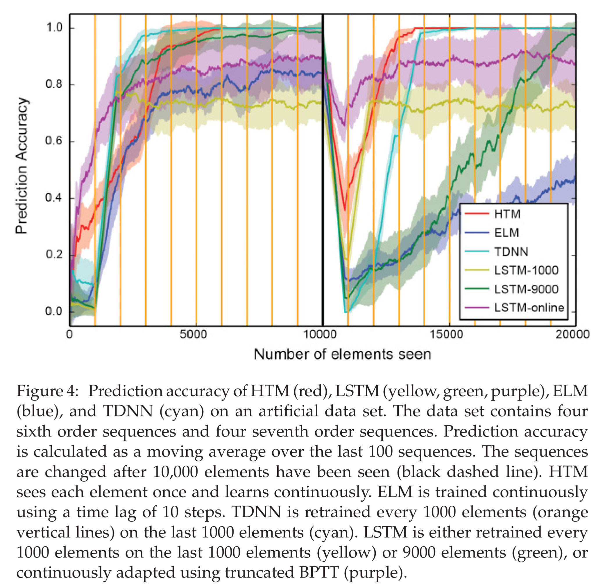
The first test compares the HTM sequence memory model with online sequential extreme machine learning (ELM), a time-delayed neural network (TDNN), and LSTMs. A data set is generated with sequences that require a network to maintain a context of at least the first two elements of a sequence in order to correctly predict the last element.
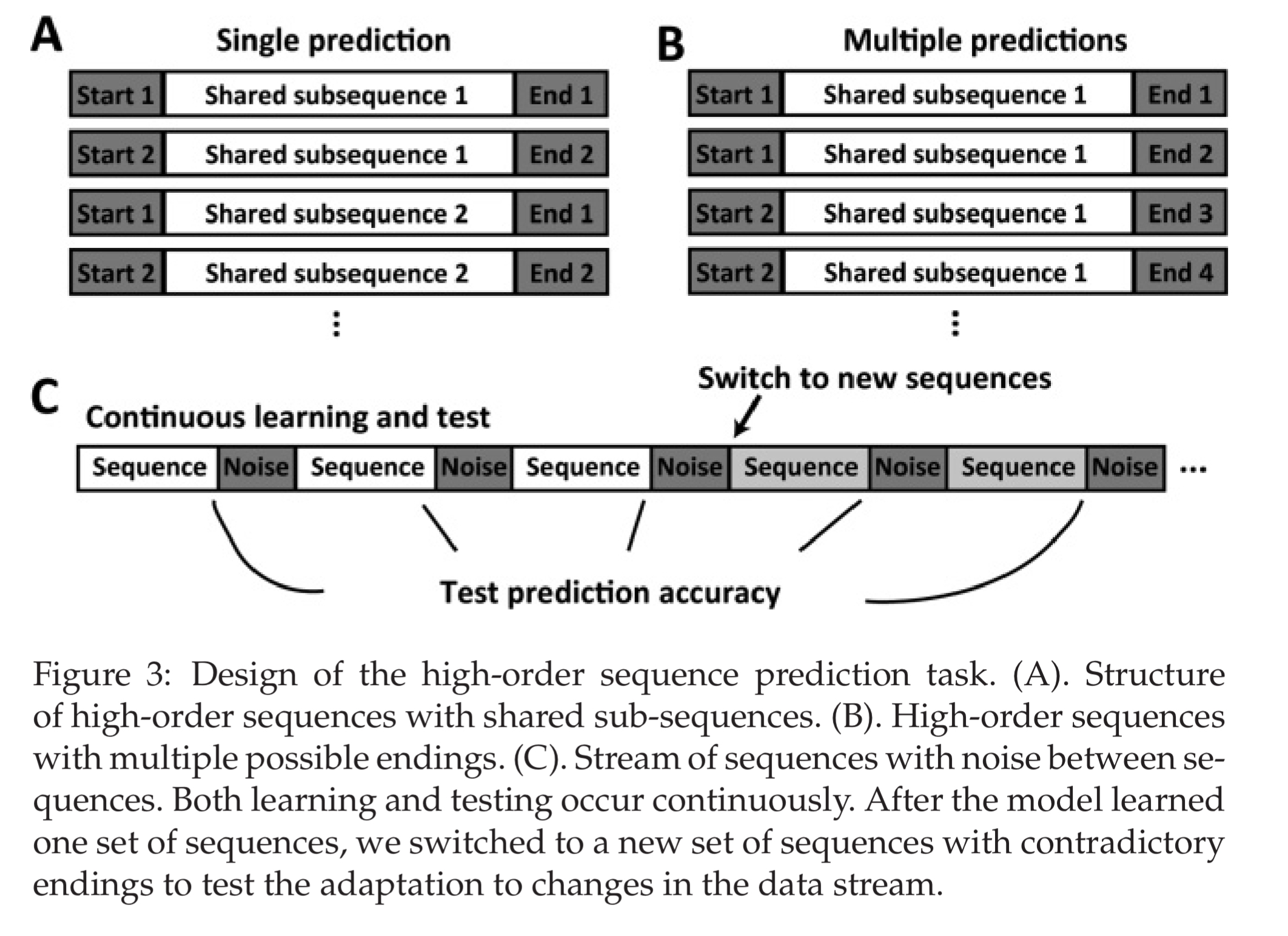
Since the sequences are presented in a streaming fashion, and predictions are required continuously, this task represents a continuous online learning problem.
For the LSTMs, retraining is done at regular intervals on a buffered data set of the previous time steps. The experiments include several LSTM models with varying buffer sizes.
In the figure below, we see the prediction accuracy achieved by the various networks when the sequences are generated such that there is a single correct prediction. After the one thousandth element, we see how quickly the networks relearn when the sequences change. HTM is not the fastest initial learner, but it does achieve full prediction accuracy and recovers accuracy fastest after the sequence change. Remember though that HTM is working online seeing each example just once, whereas the LSTM’s are periodically retrained (retraining points indicated by the vertical yellow lines in the figure below). HTMs determine the higher-order structure by themselves, whereas ELM and TDNN require the user to determine the number of steps to use as a temporal context.
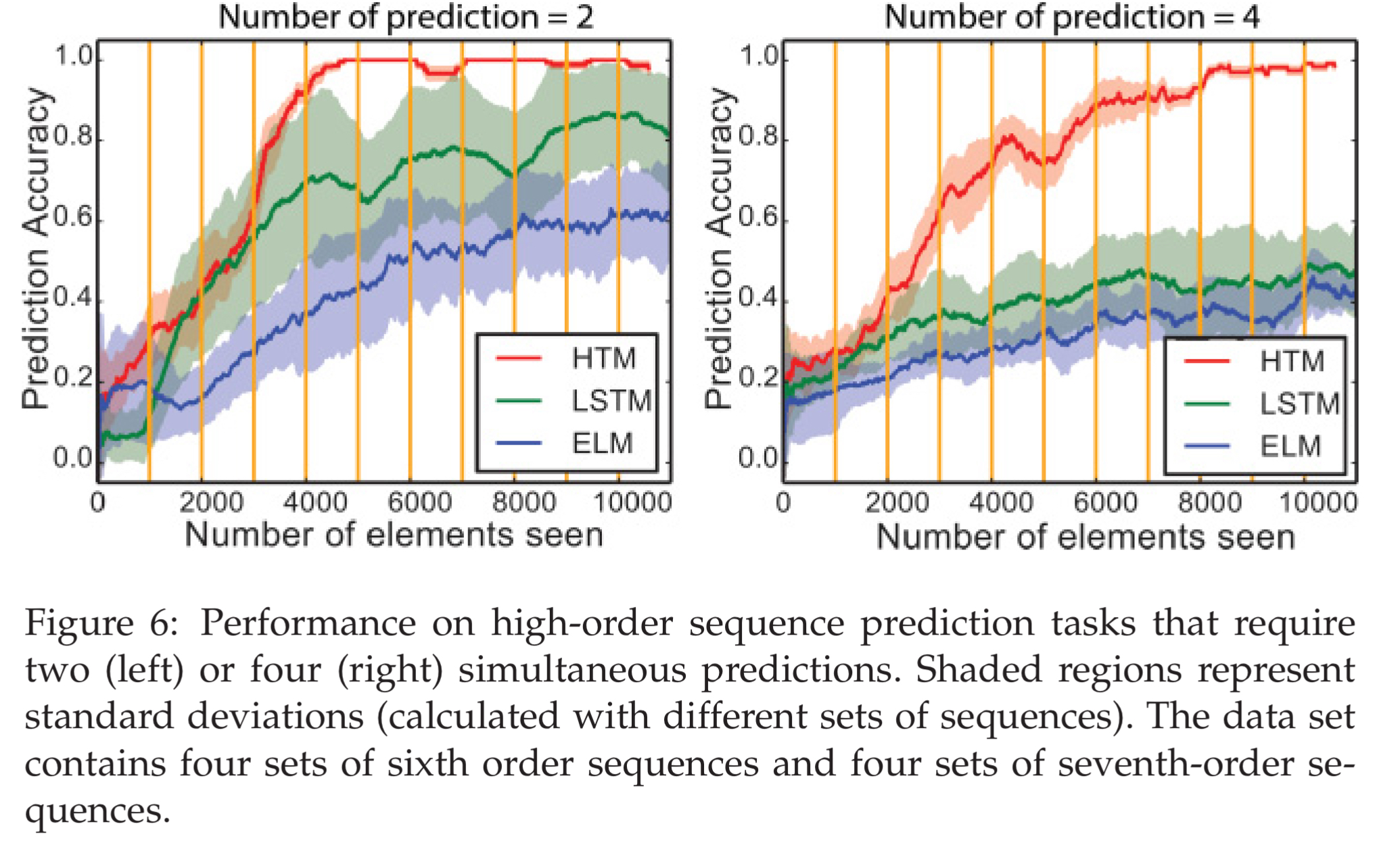
In the next experiment scenario the sequences have two or four possible endings, depending on the higher-order context. HTMs perform best at this task, and the more possible completions, the better their advantage appears to be.
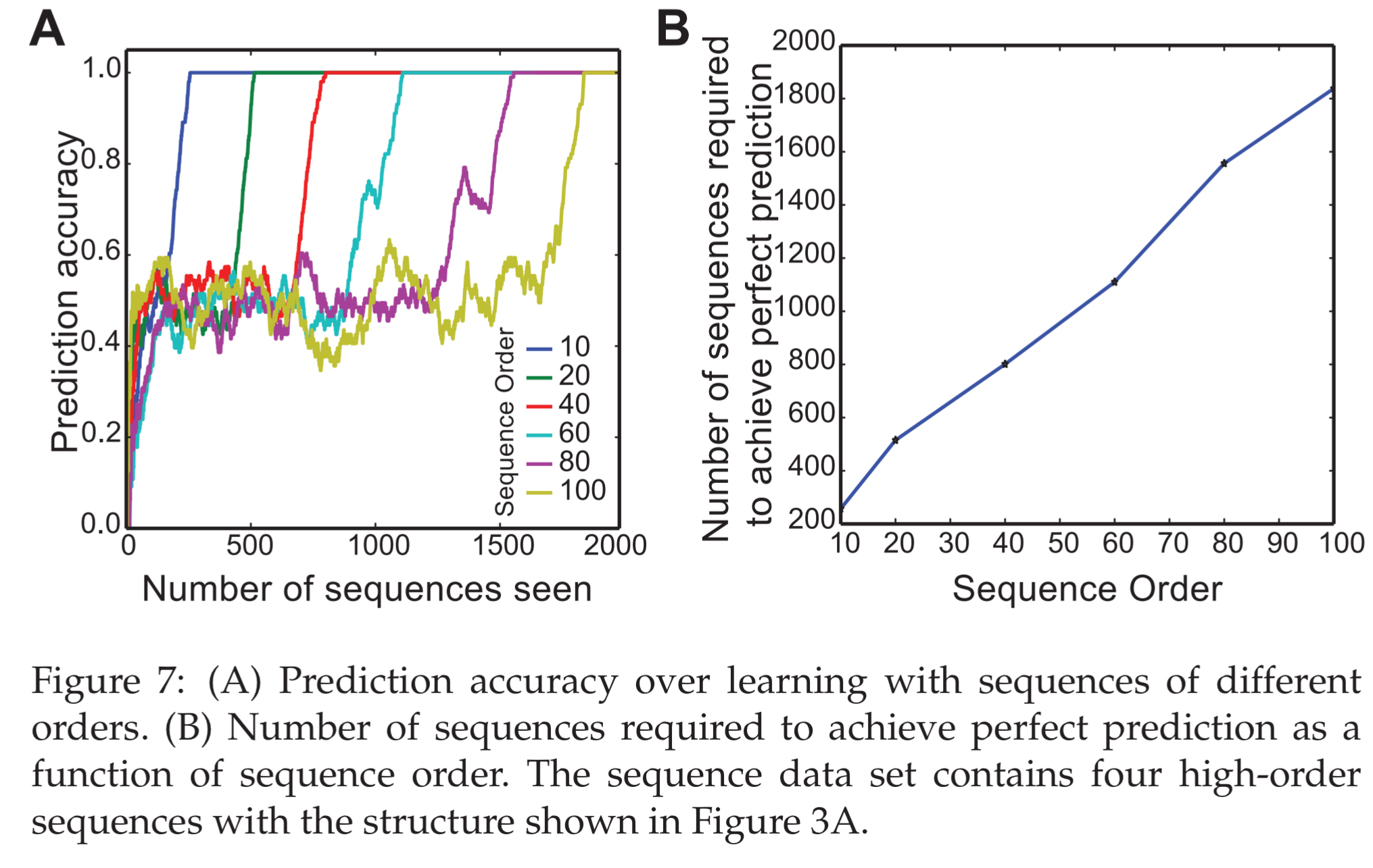
HTM sequence memory was tested with varying length sequences, and achieved perfect prediction performance up to 100-order sequences.
The number of sequences that are required to achieve perfect prediction performance increase linearly as a function of the order of sequences.
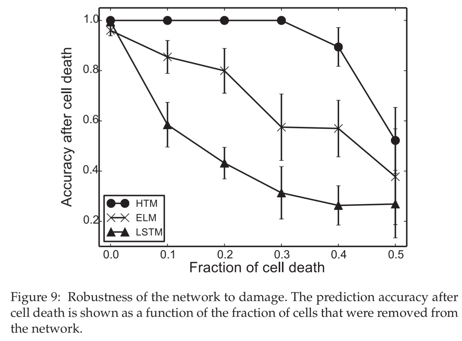
When deliberately damaging the network structure (removal of neurons), HTMs showed no impact with up to 30% cell death, whereas the ELM and LSTM networks declined more rapidly. (Techniques such as dropout were not used during training though).
New York city taxi passenger demand prediction
The HTM sequence memory model was also tested against a variety of other approaches on a task of predicting taxi demand from streaming New York City taxi ride data.
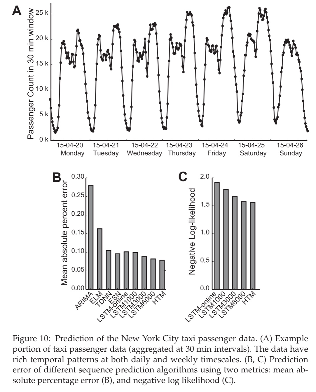
For this example, the parameters of the ESN, ELM, and LSTM network are extensively hand-tuned. The HTM model does not undergo any hyperparameter tuning.
Limitations of HTMs
We have identified a few limitations of HTM…
- As a strict one-pass algorithm with access only to the current input, it may take longer for HTM to learn sequences with very long-term dependencies than algorithms with access to a larger history buffer.
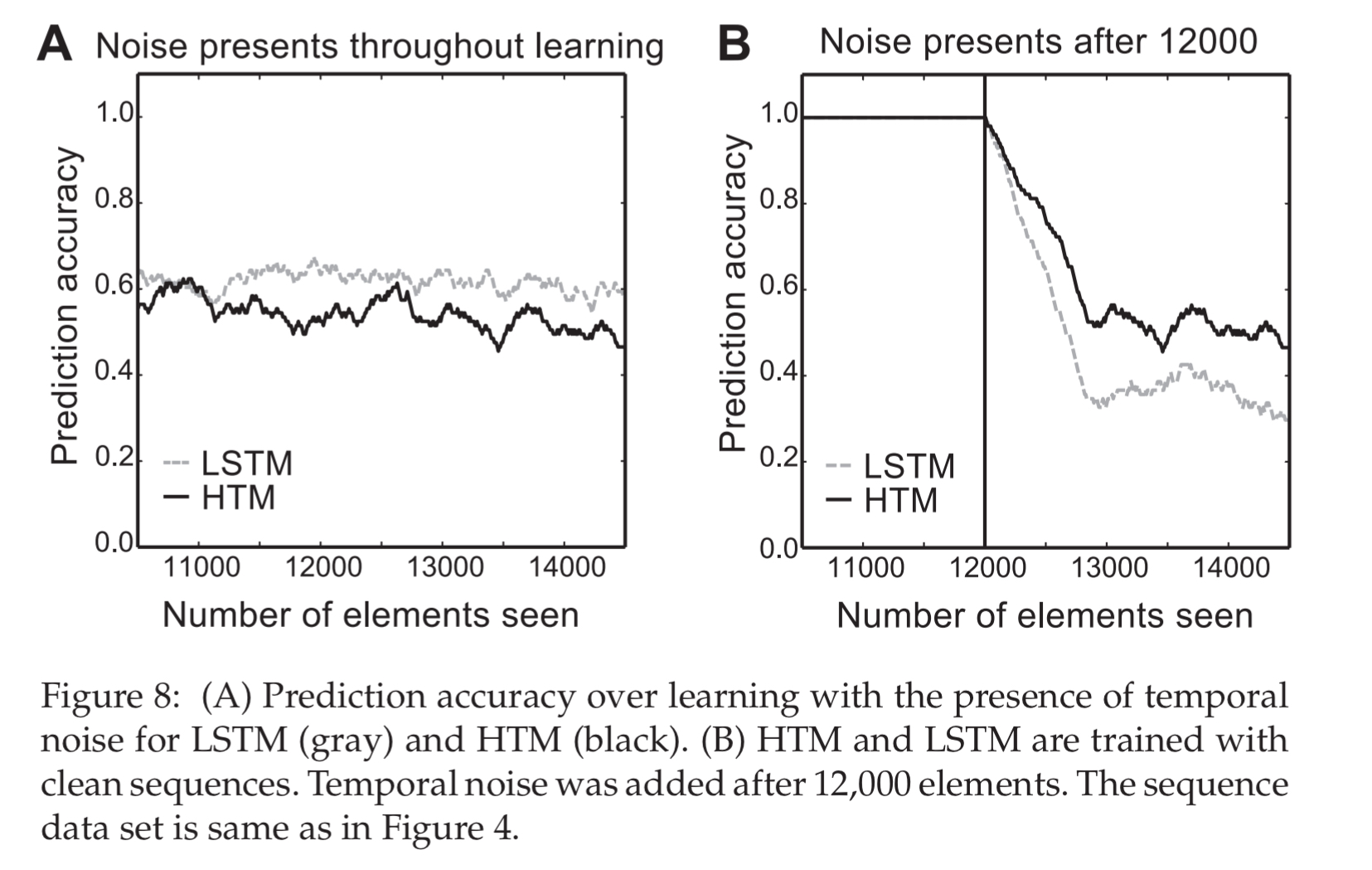
- HTM is robust to spatial noise due to the use of sparse distributed representations, but proved sensitive to temporal noise (replacing elements in a sequence by random symbols). LSTMs are more robust to temporal noise. To improve the noise robustness of HTM, a hierarchy of sequence models operating on different timescales could be used.
- The HTM model did not perform as well as LSTM on grammar learning tasks – achieving 98.4% accuracy in a test, whereas the LSTM achieves 100%.
- It is future work to determine whether HTM can handle high-dimensional data such as speech and video streams
The work on HTMs also seems to be being reported outside of the usual machine learning conference venues. It’s good to bring in ideas from further afield, but this may also mean they have received less scrutiny from the mainstream machine learning community. There has been some controversy surrounding this in the past: https://cs.stackexchange.com/questions/13089/some-criticisms-of-hierarchical-temporal-memory.