A general purpose counting filter: making every bit count Pandey et al., SIGMOD’17

It’s been a while since we looked at a full on algorithms and data structures paper, but this one was certainly worth waiting for. We’re in the world of Approximate Membership Query (AMQ) data structures, of which probably the best known example is the Bloom filter. At their core, AMQ structures allow you to track whether or not a given item is in a set. They never return false negatives (tell you that something is not in the set when in fact it is), but may return a tunable number of false positives. That is, in response to a query “is this item in the set” they return either ‘no,’ or ‘probably.’ There are variations beyond the basic membership test that also track counts of items, support deletions, allow runtime resizing of the structure, and so on.

AMQs are widely used in databases, storage systems, networks, computational biology and many other domains.

AMQs are often the computational workhorse in applications… however, many applications must work around limitations in the capabilities or performance of current AMQs, making these applications more complex and less performant.

Four important shortcomings in Bloom filters (and most production AMQs) are:

1. The inability to delete items
2. Poor scaling out of RAM
3. The inability to resize dynamically
4. The inability to count the number of occurrences of each item, especially with skewed input distributions.

This paper introduces a new AMQ data structure, a Counting Quotient Filter, which addresses all of these shortcomings and performs extremely well in both time and space: CQF performs in-memory inserts and queries up to an order of magnitude faster than the original quotient filter structure from which it takes its inspiration, several times faster than a Bloom filter, and similarly to a cuckoo filter. The CQF structure is comparable or more space efficient than all of them too. Moreover, CQF does all of this while supporting counting, outperforming all of the other forms in both dimensions even though they do not. In short, CQF is a big deal!

We’ll build up to the full CQF structure in all its glory by starting with a quick refresher on quotient filters (QF), then looking at an intermediate progression called a ‘rank-and-select-based quotient filter’ (RSQF) before going on to the full CQF.

Quotient Filters

Quotient filters support insertion, deletion, lookups, resizing, and merging. The overview on wikipedia provides a great summary. The essence of the idea is as follows:

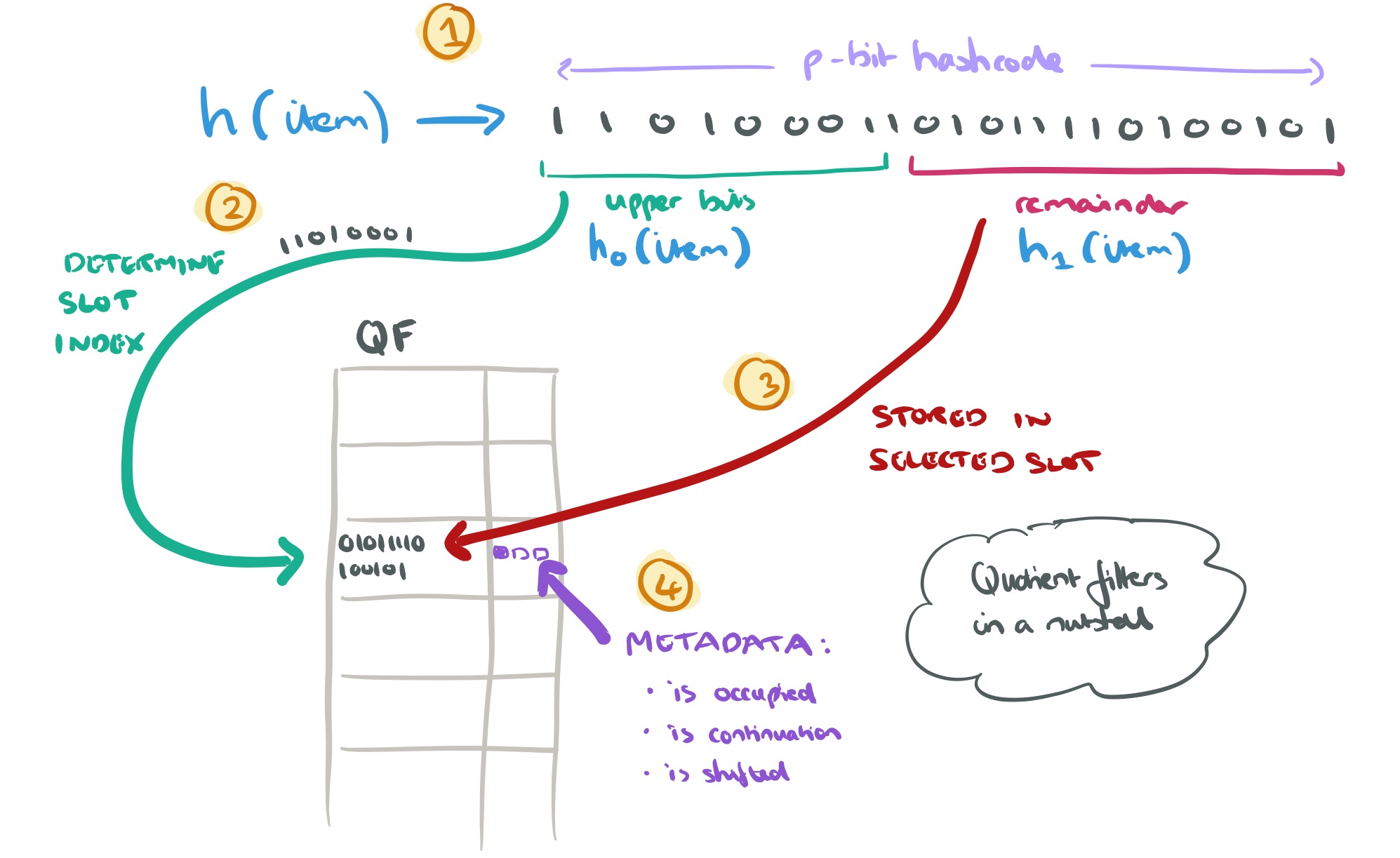
1. The item is hashed to yield a p-bit hash
2. The upper bits of the hash (denoted in the paper) are used to determine which slot in the quotient filter data structure to use
3. The remaining lower bits of the hash (denoted in the paper) are stored in the identified slot

Of course the problems come when more than one item shares the same hash upper bits, leading to a slot collision. In this case the remainder is stored in some slot to the right. This is where the quotient filter metadata data comes in. There are three bits of information tracked for each entry:

• is occupied : is this slot the canonical slot for some key stored in the filter? (Even though it may not be stored in this actual slot).
• is continuation : is this slot occupied by a remainder that is not the first entry is a run?
• is shifted : does this slot hold a remainder that is not in its canonical slot?

On lookups and inserts QF does linear probing to scan left and right in the data structure starting from the canonical slot () to find the information it needs. On insertion, elements are shifted right if need be, in order to maintain elements in increasing hash order.

The quotient filter uses slightly more space than a Bloom filter, but much less space than a counting Bloom filter, and delivers speed comparable to a Bloom filter. The quotient filter is also much more cache-friendly than the Bloom filter, and so offers much better performance when stored on SSD. One downside of the quotient filter is that the linear probing becomes expensive as the data structure becomes full – performance drops sharply after 60% occupancy.

Rank-and-Select-based Quotient Filters

Rank-and-select based quotient filters (RSQF) improve on the base QF design in three ways:

1. They use only 2.125 metadata bits per slot instead of 3
2. They support faster lookups at higher load factors than quotient filters. (Quotient filters have a recommend max utilisation of 75%, RSQFs perform well at up to 95%).
3. They store the metadata structure in such a way that bit vector rank and select operations can be used. This opens the door to optimisation using new x86 bit-manipulation instructions.

RSQF uses the same division of an item’s hash into a quotient (upper bits) used as the index of its home slot, and a remainder (lower bits) to be stored in that slot. To deal with collisions though, RSQFs track different metadata and hence uses a different form of linear probing.

• A slot i is said to be occupied if the filter contains an element x such that . (Note that with this terminology, and because of the linear probing, a slot may be in use without actually being ‘occupied’)
• A slot i is in use if there is a remainder stored in it.

RSQF always tries to put remainders in their home slots, and only shifts remainders when pushed out by other remainders. Three invariants ensure that remainders of elements with the same quotient are stored in consecutive slots (a run):

1. An occupieds bit vector is maintained in which the bit for slot i is set to 1 iff the slot is occupied.
2. If the quotient () of one item is less than the quotient of some other item y, then the remainder () is stored in an earlier slot than the remainder .
3. If a remainder for some items is stored in some slot i then its quotient is less than or equal to i, and there are no unused slots between the item’s home slot and the slot where its remainder is stored.

An RSQF also maintains a runends bit vector in which the bit for slot i is set to 1 iff the slot contains the last remainder in a run.

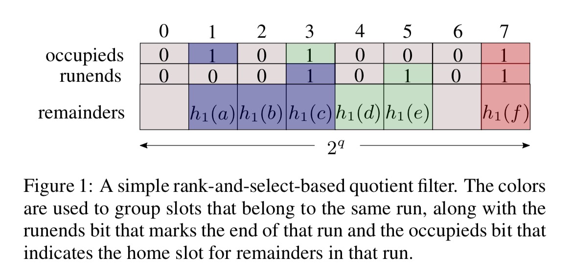
Given these data structures, bit vector rank and select operations can be used to find the run corresponding to any quotient. RANK(B,i) returns the number of 1s in B up to position i, and SELECT(B,i) returns the index of the ith 1 in B.

To find the run corresponding to any quotient :

• If the occupieds bit for is not set then no such run exists
• Otherwise, use RANK to count the number t of slots less than or equal to that have their occupied bits set. This tells us the number up to and including the home slot for x.
• Use SELECT to find the position of the _t_th runend bit, which tells us where the run of remainders with quotient ends
• Walk backwards through the remainders in that run

(See Algorithm 1 in the paper).

As expressed so far, lookups require scanning the entire data structure and are not cache-friendly (each lookup accesses the occupieds bit vector, the runends bit vector, and the remainders array).

To compute the position of a runend without scanning the entire occupieds and runends bit vectors, RSQF maintains in addition an offsets array where holds the distance from the slot i to the runend corresponding to slot i:

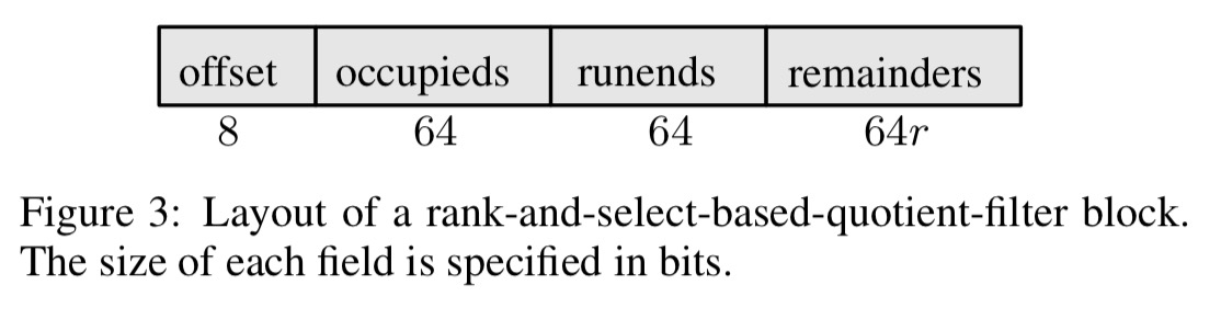
To save space, the offset is only stored for every 64th slot, with offsets for entries in-between computed at runtime. Maintaining the array of offsets is inexpensive, and computing an offset from the nearest stored offset is efficient. Offsets are stored as 8-bit unsigned ints, yielding a total metadata overhead of 2.125 bits per slot.

To make the RSQF cache efficient, we break the occupieds, runends, offsets, and remainders vectors into blocks of 64 entries, which we store together. We use blocks of 64 entries so these rank and select operations can be transformed into efficient machine-word operations.

SELECT and RANK can be efficiently implemented on 64-bit vectors using the x86 instruction set from the Haswell line of processors. SELECT is implemented using the PDEP and TZCNT instructions:

SELECT(v,i) = TZCNT(PDEP(2^i,v))

RANK is implemented using the POPCOUNT instruction:

RANK(v,i) = POPCOUNT(v & (2^i -1))

Since it is possible to enumerate the items in an RSQF, RSQFs can be resized, and they can be merged.

Merging is particularly efficient for two reasons. First, items can be inserted into the output filter in order of increasing hash value, so inserts will never have to shift any other items around. Second, merging requires only linear scans of the input and output filters, and hence is I/O-efficient when the filters are stored on disk.

Counting Quotient Filters

For the final twist, we add counting support to the RSQF structure to obtain the full Counting Quotient Filter structure, CQF.

Our counter-embedding scheme maintains the data locality of the RSQF, supports variable-sized counters, and ensures that the CQF takes no more space than an RSQF of the same multiset. Thanks to variable-size counters, the structure is space efficient even for highly skewed distributions, where some elements are observed frequently and others rarely.

The CQF maintains counts by making the remainder slots serve double duty: if a particular element occurs more than once, then the slots immediately following that element’s remainder hold an encoding of the number of times that element occurs. A CQF can tell whether a slot holds a remainder or a count since remainders are stored in increasing order, and any deviation must therefore be a count. There’s a little bit of trickiness with counts that span more than one slot, and remainders that are zero – see section 4 in the paper for the details.

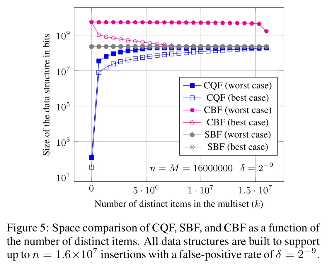
Figure 5 below shows the space bounds for CQF as a function of the number of distinct items. Even the worst case for CQF is better than the best-case space usage of the other data structures for almost all values of k.

CQFs can be made multithreaded (thread-safe) by dividing the CFQ into regions of 4096 contiguous slots. Inserts lock two consecutive regions (the region in which the item hashes, and the one following). If queries can tolerate slightly stale date – for example, applications which have an insert phase followed by a query phase – then items can be inserted in a thread-local CQF if a lock cannot be obtained on the first attempt. The local CQF is dumped into the main CQF when it fills up.

Key performance results

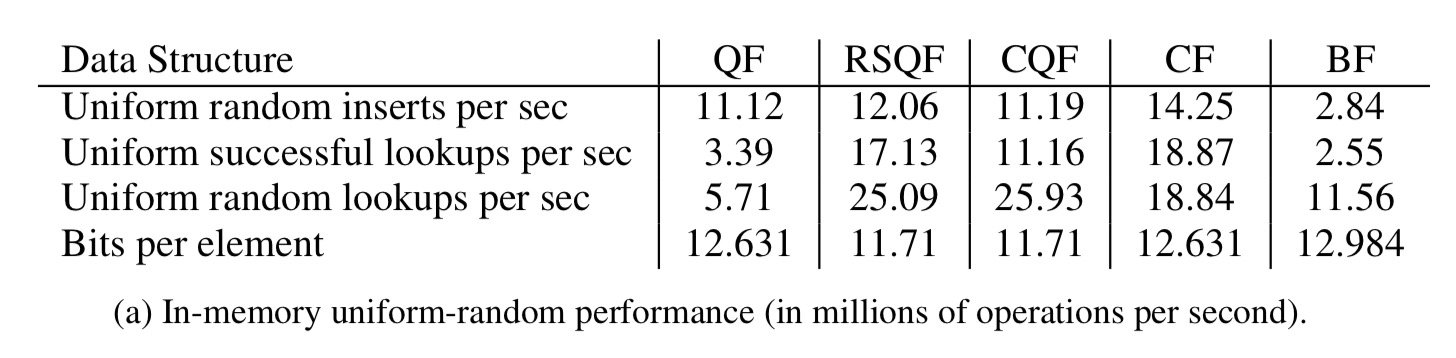
The evaluation compares RSQF and CQF performance against a state-of-the-art Bloom filter, the base Quotient Filter (QF), Cuckoo Filters (CF), and Counting Bloom Filters (CBF). The short version is that RSQF and CQF perform very well across the board.

In our experiments, the CQF performs in-memory inserts and queries up to an order-of-magnitude faster than the original filter, several times faster than a Bloom filter, and similarly to the cuckoo filter, even though none of these other data structures support counting. On SSD, the CQF outperforms all structures by a factor of at least 2 because the CQF has good data locality.

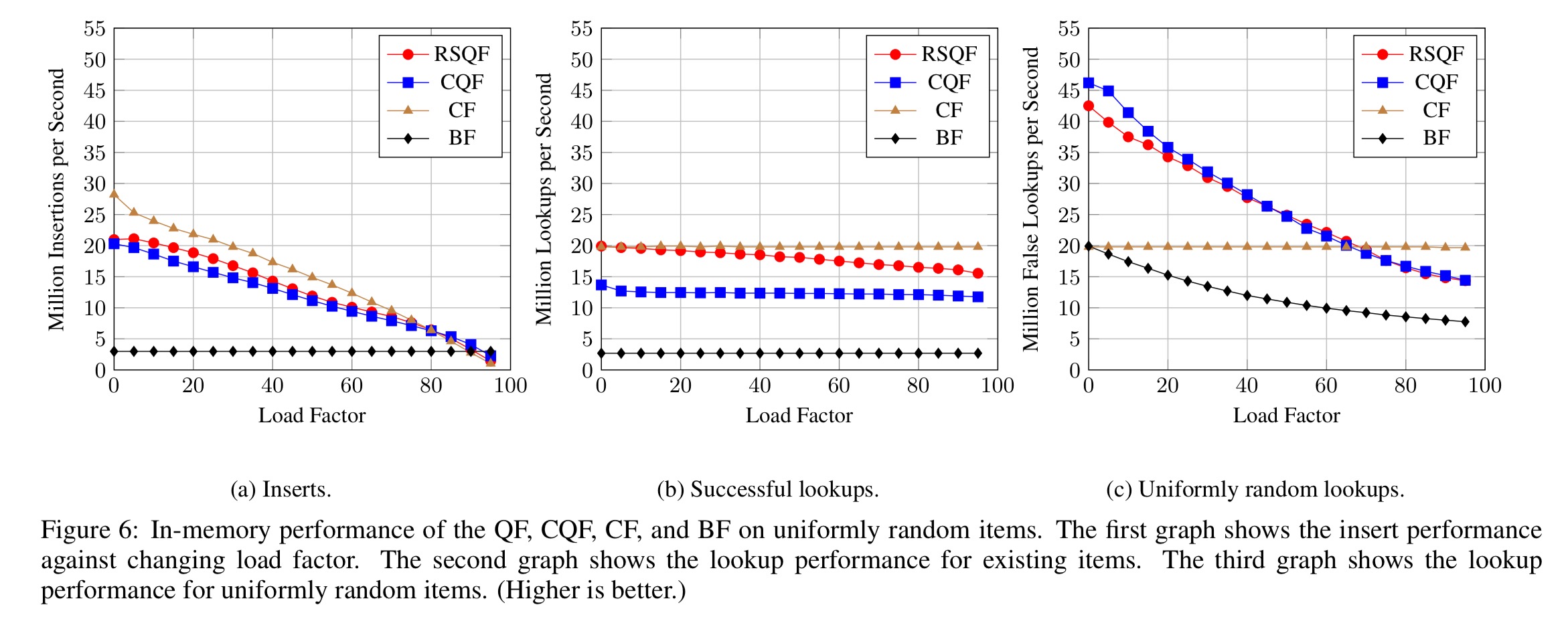
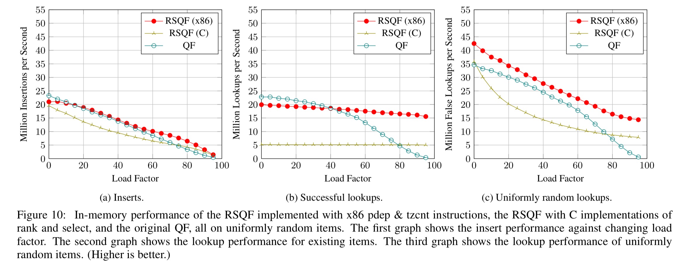
Here are the key results for in-memory performance with a uniform random item distribution:

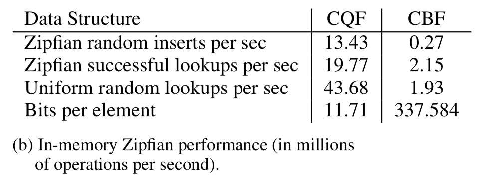
And if we make the item distribution Zipfian instead:

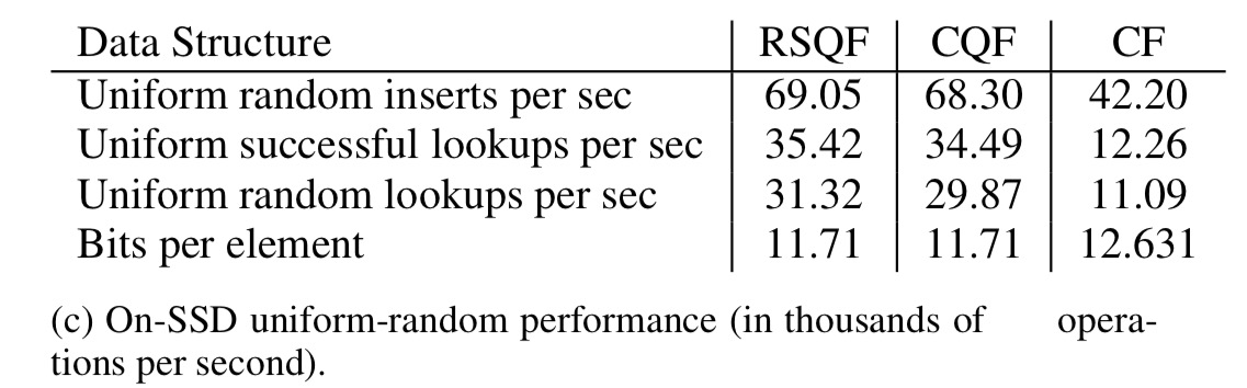
Or if we store the structure on SSDs:

The following charts show the impact of the x86 bit-vector instructions:

This paper shows that it is possible to build a counting data structure that offers good performance and saves spaces, regardless of the input distribution. Our counting quotient filter uses less space than other counting filters, and in many cases uses less space than non-counting, membership-only data structures.