End-to-end optimized image compression Ballé et al., ICLR’17
We’ll be looking at some of the papers from ICLR’17 this week, starting with “End-to-end optimized image compression” which makes a nice comparison with the Dropbox JPEG compression paper that we started with last week. Of course you won’t be surprised to find out that the authors of an ICLR paper set up a system to learn an efficient coding scheme. Covering this paper is a bit of a stretch goal for me in terms of my own understanding of some of the background, but I’m going to give it my best shot!
As we saw in that paper last week, we typically use a probabilistic encoding scheme (i.e., things that occur most frequently in the chosen representation get encoded using the fewest bits…) for image compression. Or as Ballé et al. put it:
Data compression is a fundamental and well-studied problem in engineering, and is commonly formulated with the goal of designing codes for a given discrete data ensemble with minimal entropy. The solution relies heavily on knowledge of the probabilistic structure of the data, and thus the problem is closely related to probabilistic source modeling.
A code can only map to and from a finite set of values, so any continuous data (e.g., real numbers) must be quantized to some finite set of discrete values (e.g., an integer range). As we’ll see soon, all this fancy talk of “quantizing” actually equates to the simple operation of rounding to the nearest integer in this instance. However you choose to quantize, you’re going to lose some information, which introduces error in the image reconstruction.
In this context, known as the lossy compression problem, one must trade-off two competing costs: the entropy of the discretized representation (rate) and the error arising from the quantization (distortion).
Or as you and I might express it: you have to trade-off between compressed image size and image quality.
A typical image compression scheme has three phases, using what is known as transform coding:
- Linearly transform the raw data into a suitable continuous-valued representation. JPEG uses a discrete cosine transformation on blocks of pixels, and JPEG 2000 (which gives better looking image results, but is not widely deployed in practice) uses a multi-scale orthogonal wavelet decomposition.
- Quantize the elements of the representation independently (map them to a finite number of buckets).
- Encode the resulting discrete representation using a lossless entropy code.
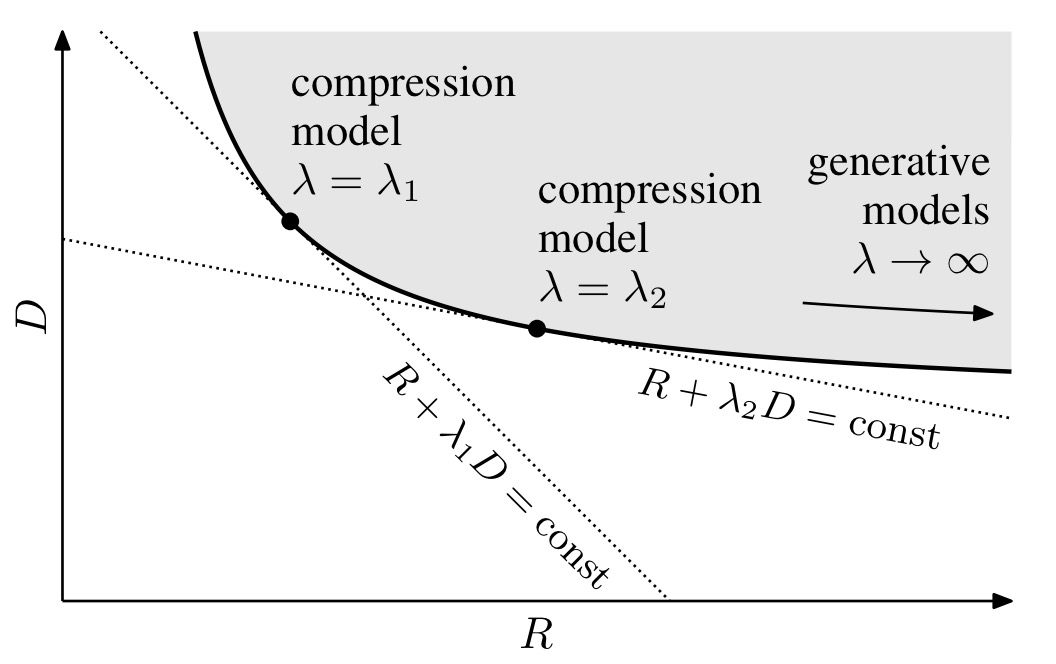
Jointly optimising both rate and distortion (size and quality) is known to be difficult. In this paper the authors develop a framework for end-to-end optimisation of an image compression model based on nonlinear transforms. The parameters of the model are learned using stochastic gradient descent, optimising for any desired point along the rate-distortion curve.
The big (and the not-so-big!) picture
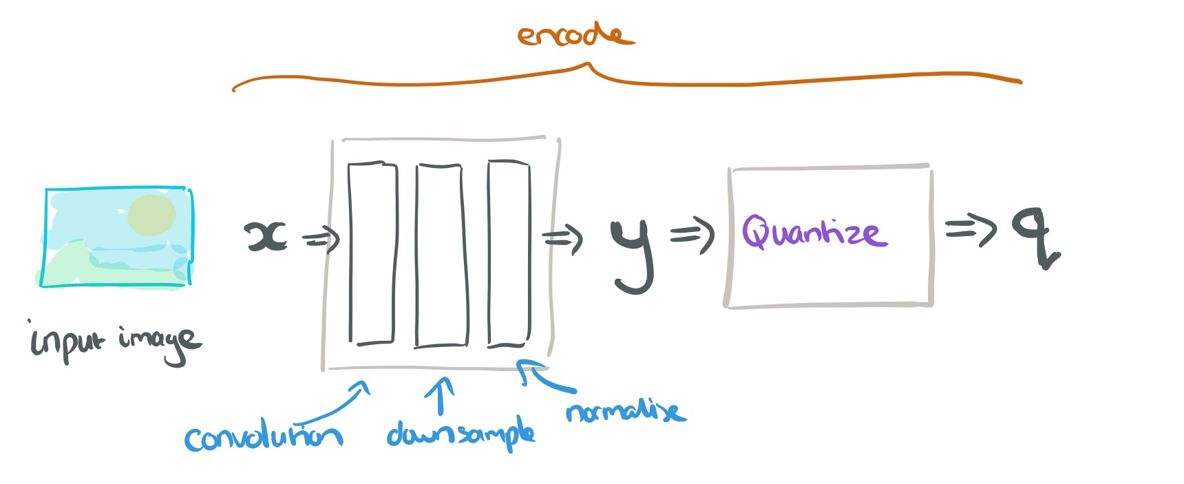
The basic structure looks like an autoencoder. We start with an input vector 


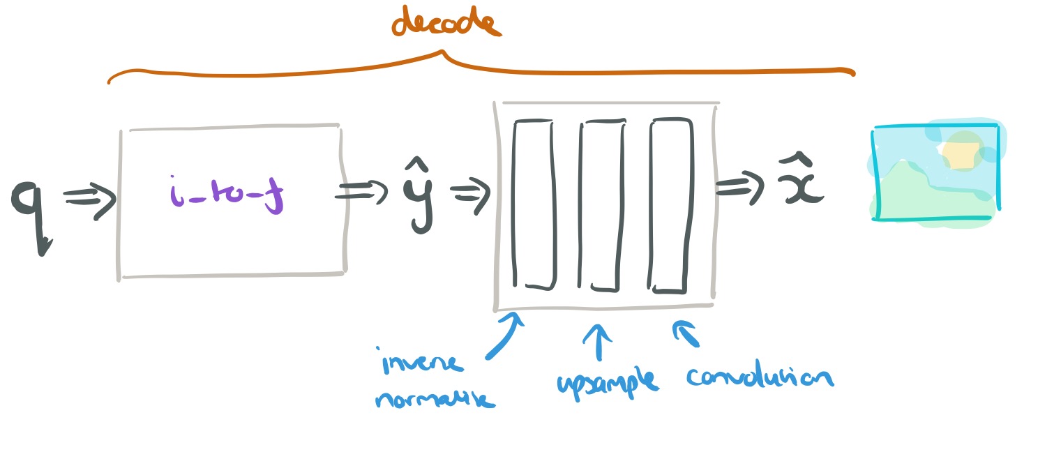
To reverse the process, the discrete representation 
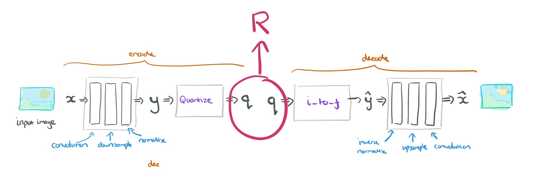
If we put these two processes back-to-back, we can see that
To measure the distortion, D both the original input image and the output synthesized image are transformed to a perceptual space using a fixed transform, and we take the difference in the perceptual space. In principle you could use a number of different perceptual transforms, but in this work the authors simply use the identity function (so really we could just have ignored the perceptual transform bit). For difference between 

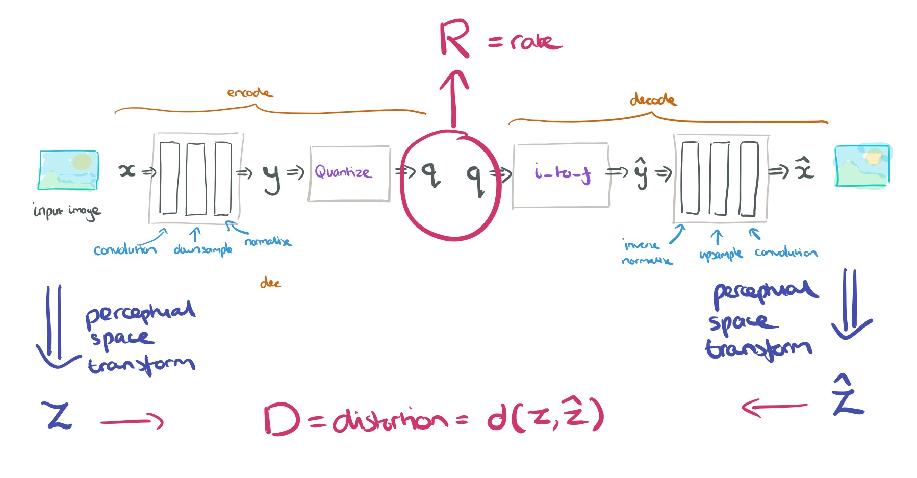
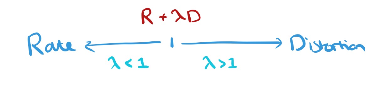
The system is trained end-to-end, and since we want to jointly optimise both rate and distortion, we set things up to optimise 

Inside the analysis transform
The analysis transform actually chains together three iterations (stages) of convolution, downsampling, and normalisation (GDN) as shown below:
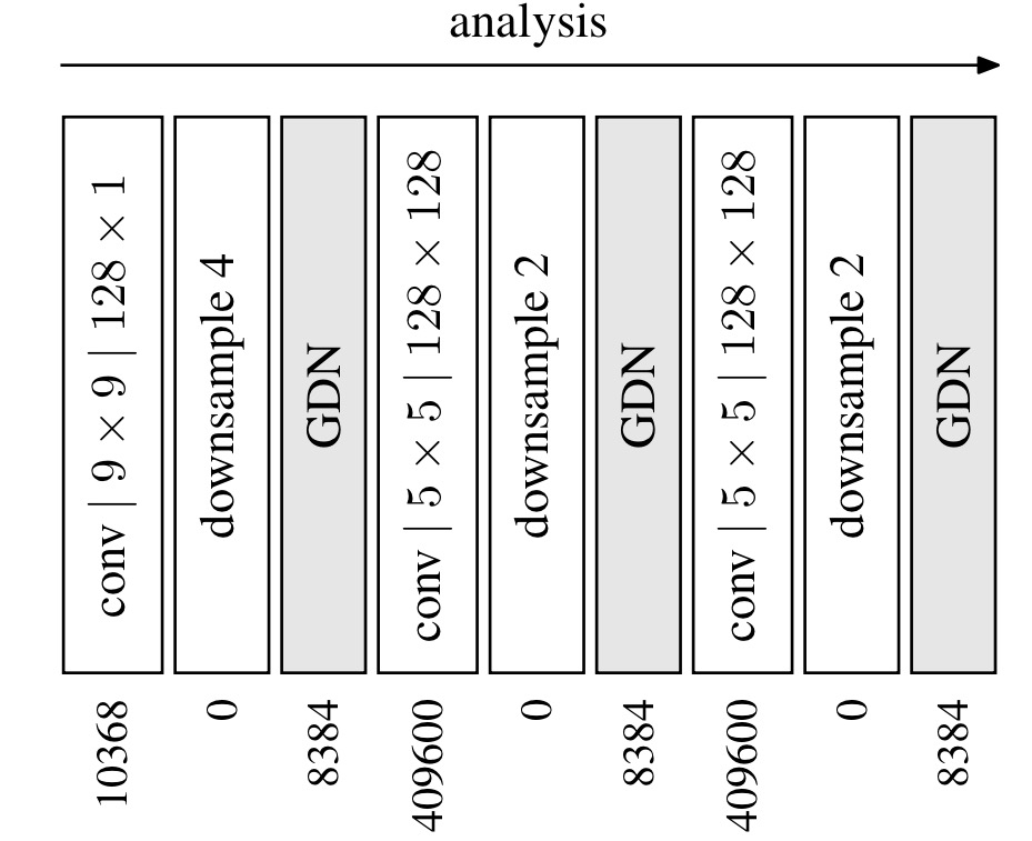
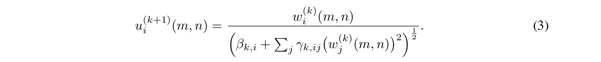
GDN stands for generalized divisive normalisation, “which has previously been shown to be highly efficient in Gaussianizing the local joint statistics of natural images.” Gaussianizing here means mapping the data onto a normal distribution. The normalisation operation looks like this, where }(m,n)")
")


Inside the synthesis transform
The synthesis transform reverses the analysis transform with a mirror network:
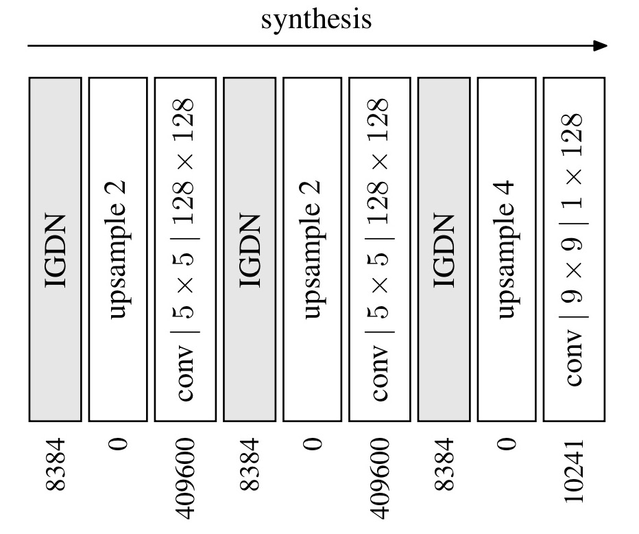
Here GDN is replaced by an approximate inverse the authors call IGDN.

Loss function
Our objective is to minimize a weighted sum of the rate and distortion,
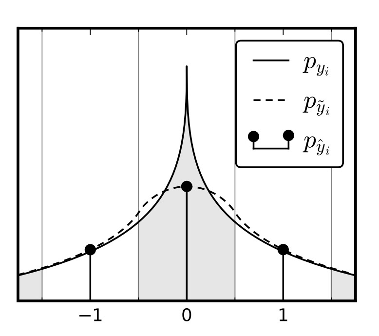
Since the actual rates achieved by an entropy code are only slightly larger than the entropy, the objective (loss) function can be defined directly in terms of entropy. Both the rate and distortion terms depend on quantized values, and the derivatives of the quantization function (i.e., rounding the nearest integer) are zero almost everywhere.
To allow optimization via stochastic gradient descent, we replace the quantizer with an additive i.i.d. uniform noise source
, which has the same width as the quantization bins (1).
The density function of 
Experimental results
Training was performed over a subset of 6507 images from the ImageNet database, for a variety of
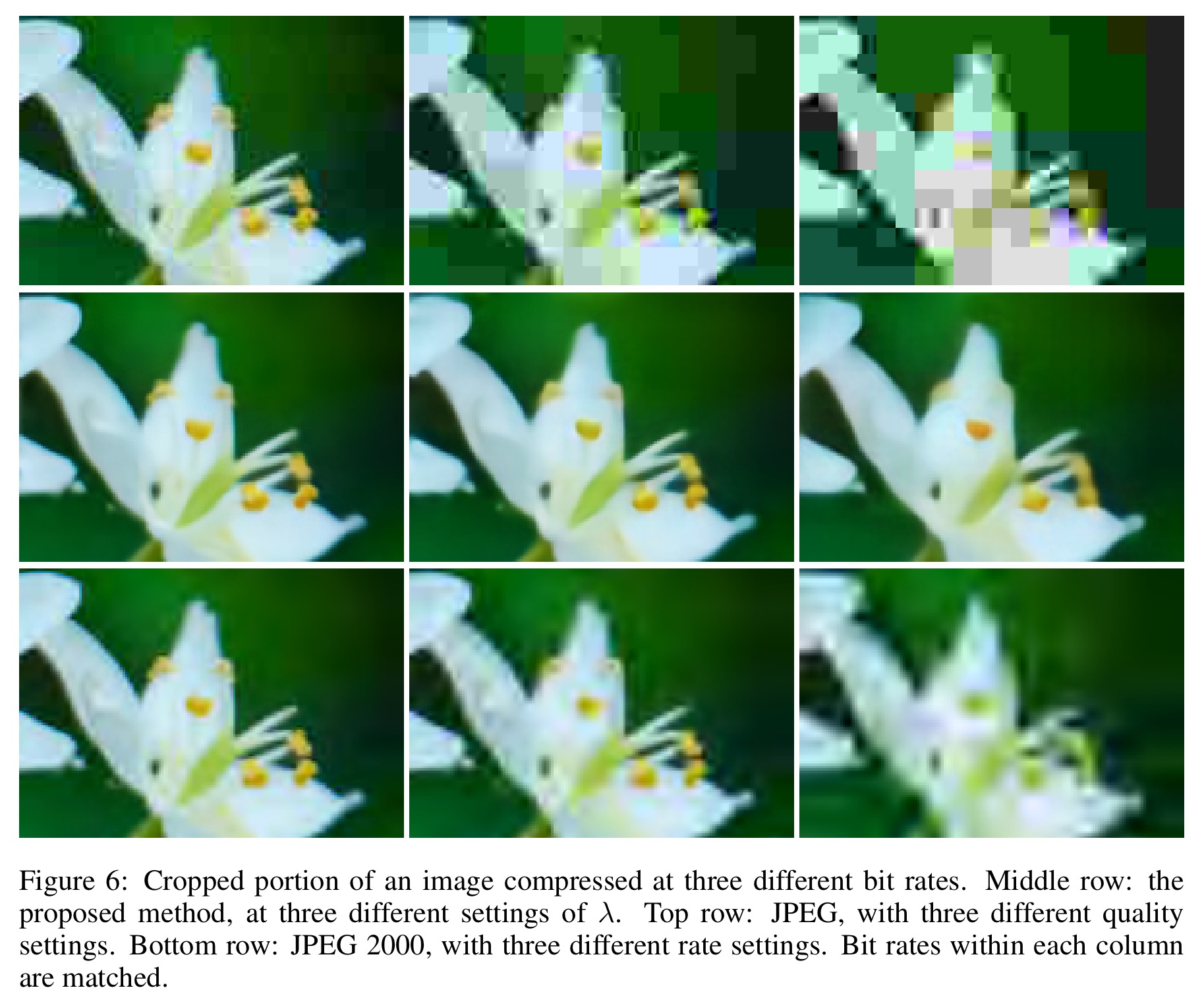
Here’s an example comparing the three approaches across each of three different image sizes:
And here’s another example with a 752×376 image:
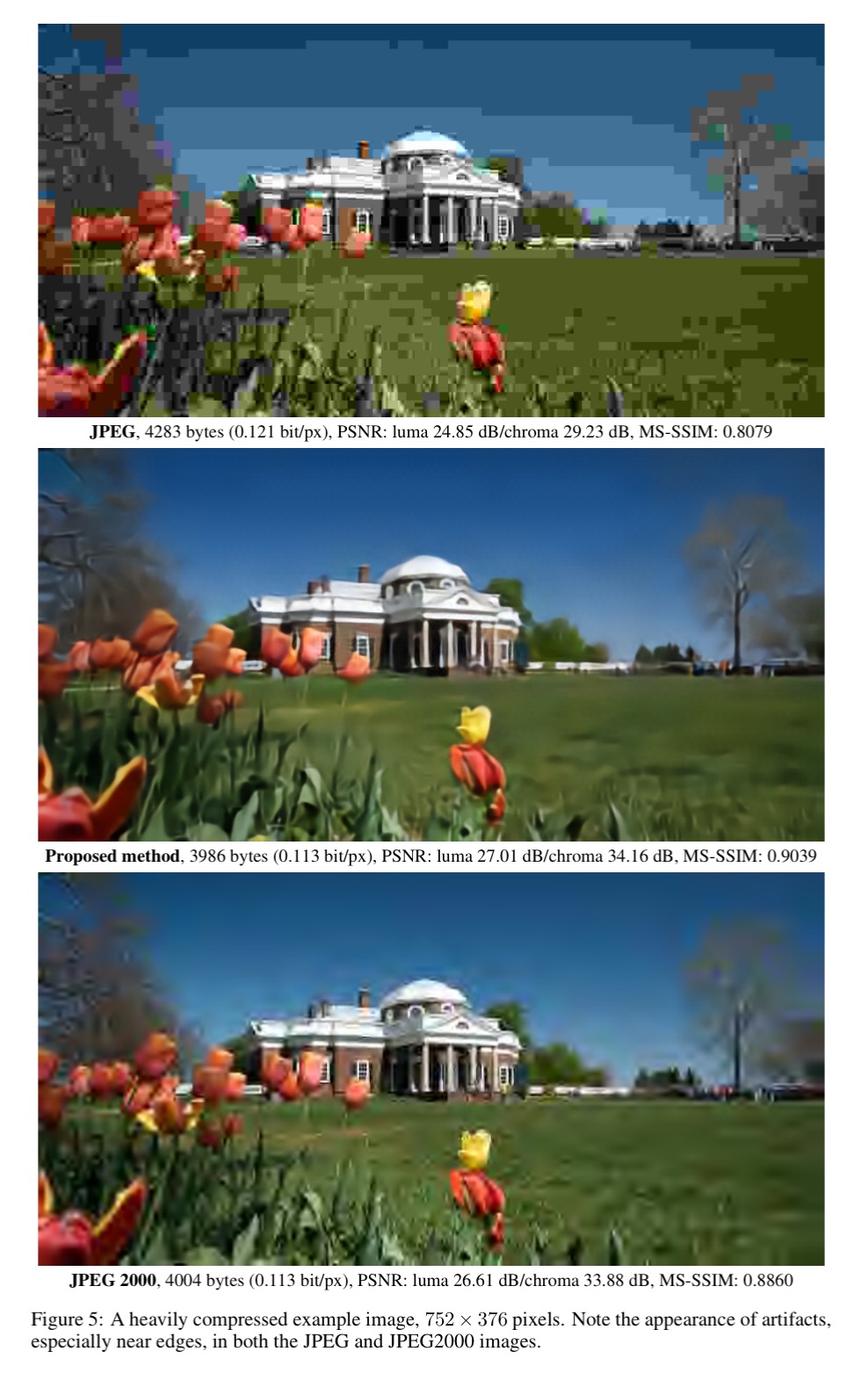
The image compressed with our method have less detail than the original (not shown, but available online), with fine texture and other patterns often eliminated altogether, but this is accomplished in a way that preserves the smoothness of contours and sharpness of many of the edges, giving them a natural appearance.
In contrast, the linear coding methods of JPEG and JPEG 2000 produce visually disturbing blocking, aliasing, and ringing artifacts reflecting the underlying basis functions.
Remarkably, we find that the perceptual advantages of our method hold for all images tested, and at all bit rates… our method appears to progressively simplify contours and other image features, effectively concealing the underlying quantization of the representation.