To round out the week, I thought I’d take a selection of fun papers from the ‘More papers from 2016’ section of top 100 awesome deep learning papers list.
- Colorful image colorization, Zhang et al., 2016
- Texture networks: feed-forward synthesis of textures and stylized images
- Generative visual manipulation on the natural image manifold, Zhu et al., 2016
- WaveNet: a generative model for raw audio, van den Oord et al., 2016
- Google’s neural machine translation system: bridging the gap between human and machine translation, Wu et al., 2016
The texture networks paper we’ve covered before, so the link in the above list is to The Morning Paper write-up (but I felt like it belonged in this group nevertheless).
Colorful image colorization
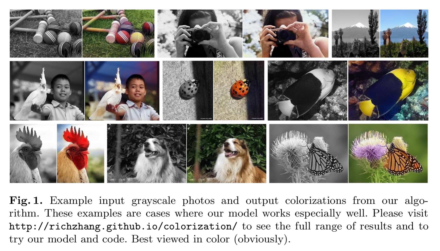
Given a grayscale photograph as input, this paper attacks the problem of hallucinating a plausible color version of the photograph.
How is this possible? Well, we’ve seen that networks can learn what various parts of the image represent. If you see enough images you can learn that grass is (usually) green, the sky is (sometimes!) blue, and ladybirds are red. The network doesn’t have to recover the actual ground truth colour, just a plausible colouring.
Therefore, our task becomes much more achievable: to model enough of the statistical dependencies between the semantics and the textures of grayscale images and their color versions in order to produce visually compelling results.
Results like this:
Training data for the colourisation task is plentiful – pretty much any colour photo will do. The tricky part is finding a good loss function – as we’ll see soon, many loss functions produce images that look desaturated, whereas we want vibrant realistic images.
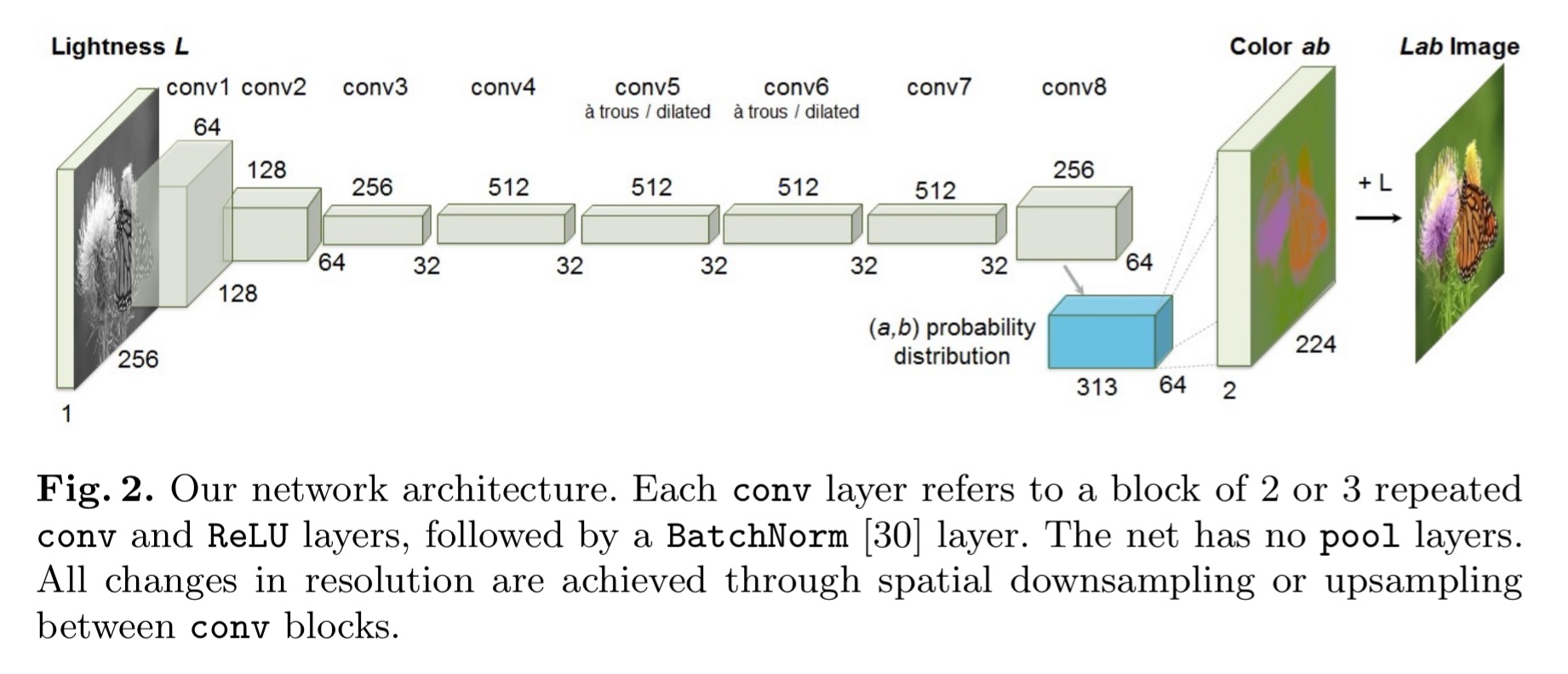
The network is based on image data using the CIE Lab colourspace. Grayscale images have only the lightness, L, channel, and the goal is to predict the a (green-red) and b (blue-yellow) colour channels. The overall network architecture should look familiar by now, indeed so familiar that supplementary details are pushed to an accompanying website.
(That website page is well worth checking out by the way, it even includes a link to a demo site on Algorithmia where you can try the system out for yourself on your own images).
Colour prediction is inherently multi-modal, objects can take on several plausible colourings. Apples for example may be red, green, or yellow, but are unlikely to be blue or orange. To model this, the prediction is a distribution of possible colours for each pixel. A typical objective function might use e.g. Euclidean loss between predicted and ground truth colours.
However, this loss is not robust to the inherent ambiguity and multimodal nature of the colorization problem. If an object can take on a set of distinct ab values, the optimal solution to the Euclidean loss will be the mean of the set. In color prediction, this averaging effect favors grayish, desaturated results. Additionally, if the set of plausible colorizations is non-convex, the solution will in fact be out of the set, giving implausible results.
What can we do instead? The ab output space is divided into bins with grid size 10, and the top Q = 313 in-gamut (within the range of colours we want to use) are kept:
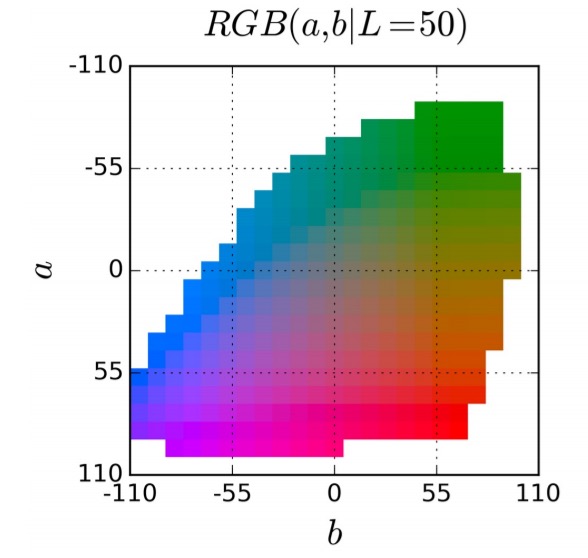
The network learns a mapping to a probability distribution over these Q colours (a Q-dimensional vector). The ground truth colouring is also translated into a Q-dimensional vector, and the two are compared using a multinomial cross entropy loss. Notably this includes a weighting term to rebalance loss based on colour-class rarity.
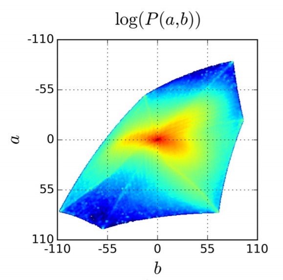
The distribution of ab values in natural images is strongly biased towards values with low ab values, due to the appearance of backgrounds such as clouds, pavement, dirt, and walls. Figure 3(b) [below] shows the empirical distribution of pixels in ab space, gathered from 1.3M training images in ImageNet. Observethat the number of pixels in natural images at desaturated values are orders of magnitude higher than for saturated values. Without accounting for this, the loss function is dominated by desaturated ab values.
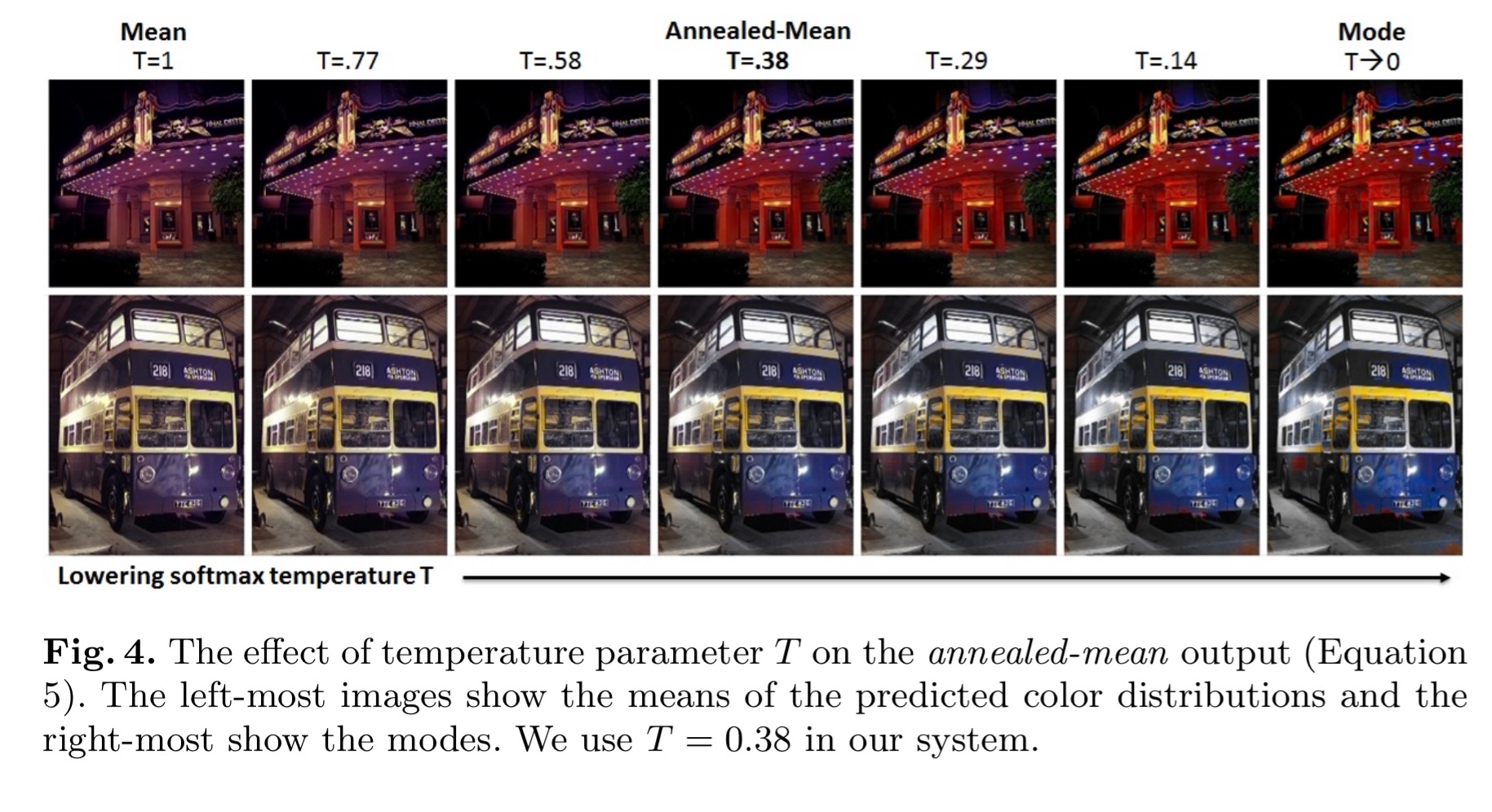
The final predicted distribution then needs to be mapped to a point estimated in ab space. Taking the mode of the predicted distribution leads to vibrant but sometimes spatially inconsistent results (see RH column below). Taking the mean brings back another form of the desaturation problem (see LH column below).
To try to get the best of both worlds, we interpolate by re-adjusting the temperature T of the softmax distribution, and taking the mean of the result. We draw inspiration from the simulated annealing technique, and thus refer to the operation as taking the annealed-mean of the distribution.
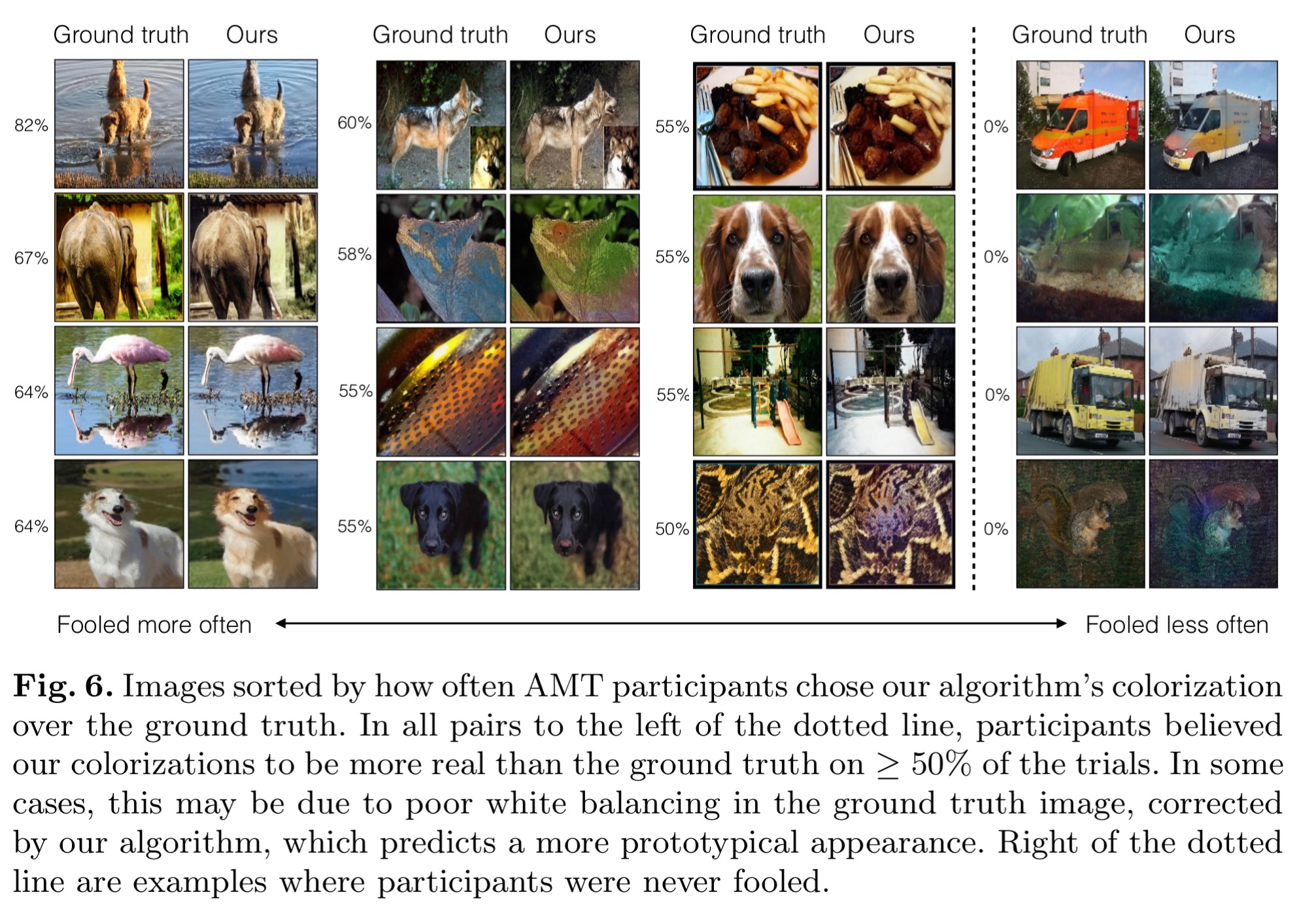
Here are some more colourings from a network trained on ImageNet, which were rated by Amazon Mechanical Turk participants to see how lifelike they are.
And now for my very favourite part of the paper:
Since our model was trained using “fake” grayscale images generated by stripping ab channels from color photos, we also ran our method on real legacy black and white photographs, as shown in Figure 8 (additional results can be viewed on our project webpage). One can see that our model is still able to produce good colorizations, even though the low-level image statistics of the legacy photographs are quite different from those of the modern-day photos on which it was trained.
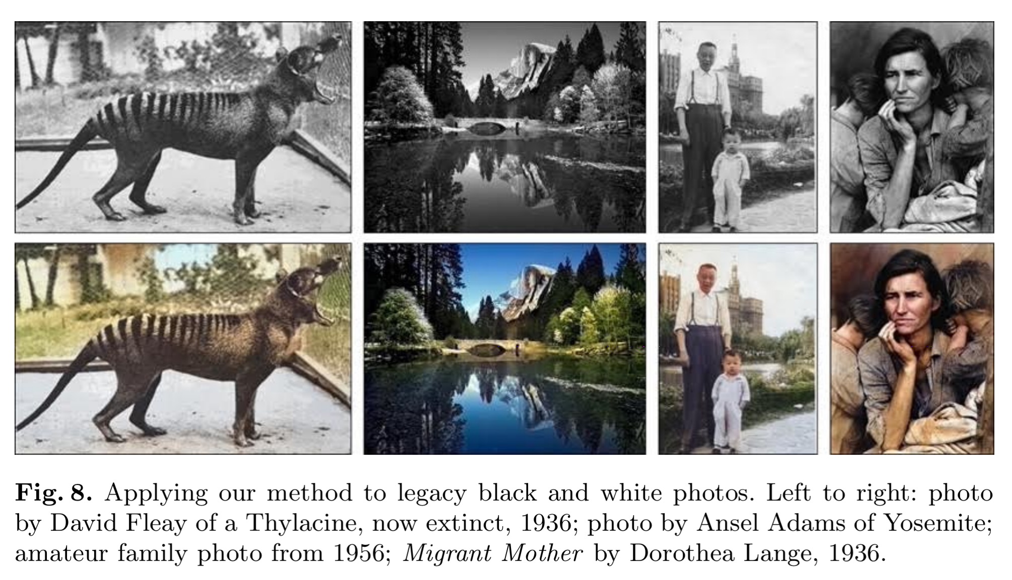
Aren’t they fabulous! Especially the Migrant Mother colouring.
The representations learned by the network also proved useful for object classification, detection, and segmentation tasks.
Generative visual manipulation on the natural image manifold
So we’ve just seen that neural networks can help us with our colouring. But what about those of us that are more artistically challenged and have a few wee issues making realistic looking drawings (or alterations to existing drawings) in the first place? In turns out that generative adversarial neural networks can help.
It’s a grand sounding paper title, but you can think of it as “Fiddling about with images while ensuring they still look natural.” I guess that wouldn’t look quite so good in the conference proceedings ;).
Today, visual communication is sadly one-sided. We all perceive information in the visual form (through photographs, paintings, sculpture, etc), but only a chosen few are talented enough to effectively express themselves visually… One reason is the lack of “safety wheels” in image editing: any less-than-perfect edit immediately makes the image look completely unrealistic. To put another way, classic visual manipulation paradigm does not prevent the user from “falling off” the manifold of natural images.
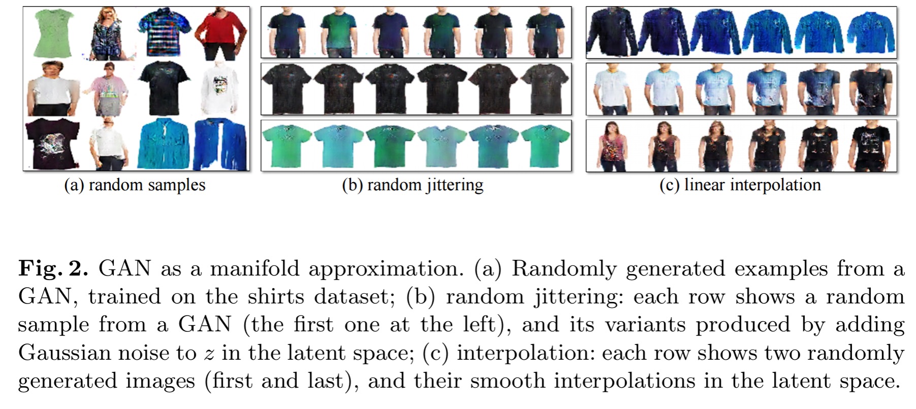
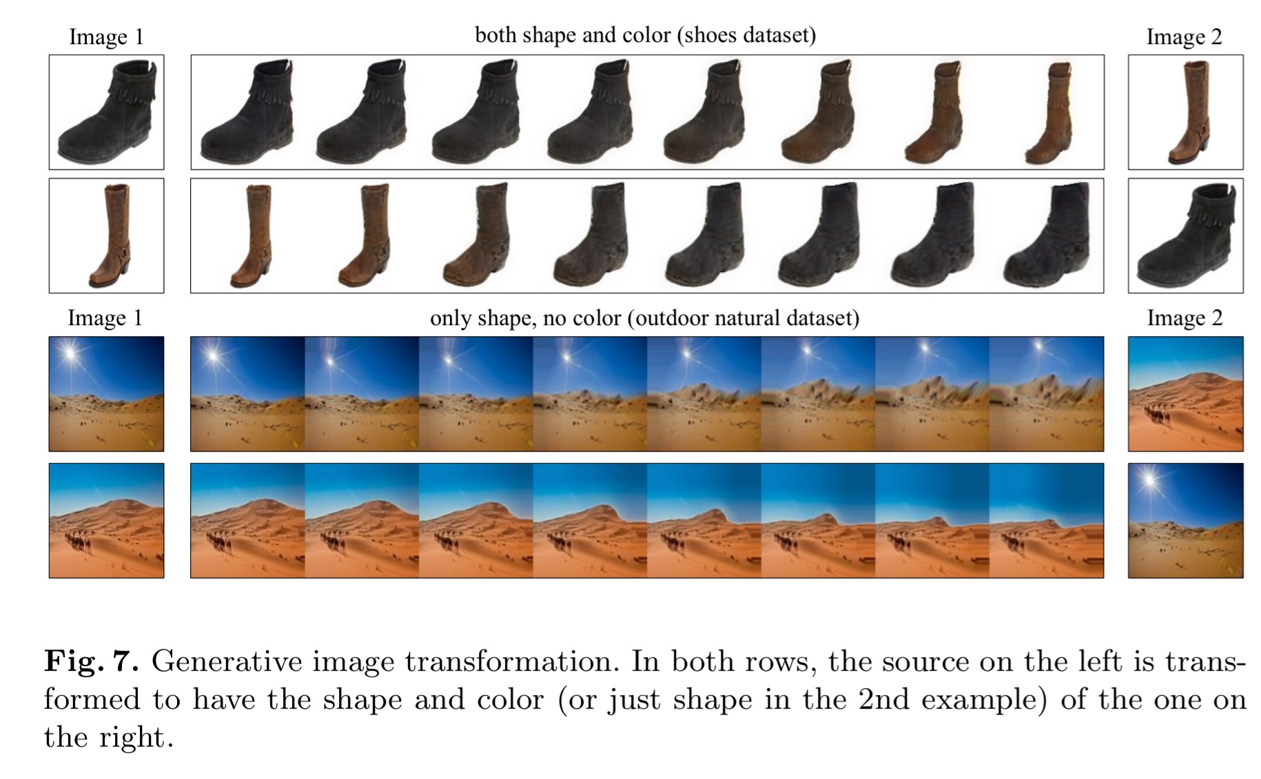
As we know, GANs can be trained to learn effective representations of natural looking images (“the manifold of natural images“). So let’s do that, but then instead of using the trained GAN to generate images, use it as a constraint on the output of various image manipulation operations, to make sure the results lie on the learned manifold at all times. The result is an interactive tool that helps you make realistic looking alterations to existing images. It helps to see the tool in action, you can see a video here. The authors also demonstrate ‘generative transformation’ of one image to look more like another, and my favourite, creating a new image from scratch based on a user’s sketch.
The intuition for using GANs to learn manifold approximations is that they have been shown to produce high-quality samples, and that Euclidean distance in the latent space often corresponds to a perceptually meaningful visual similarity. This means we can also perform interpolation between points in the latent space.
Here’s what happens when the latent vector is updated based on user edits (top row, adding black colour and changing the shape):
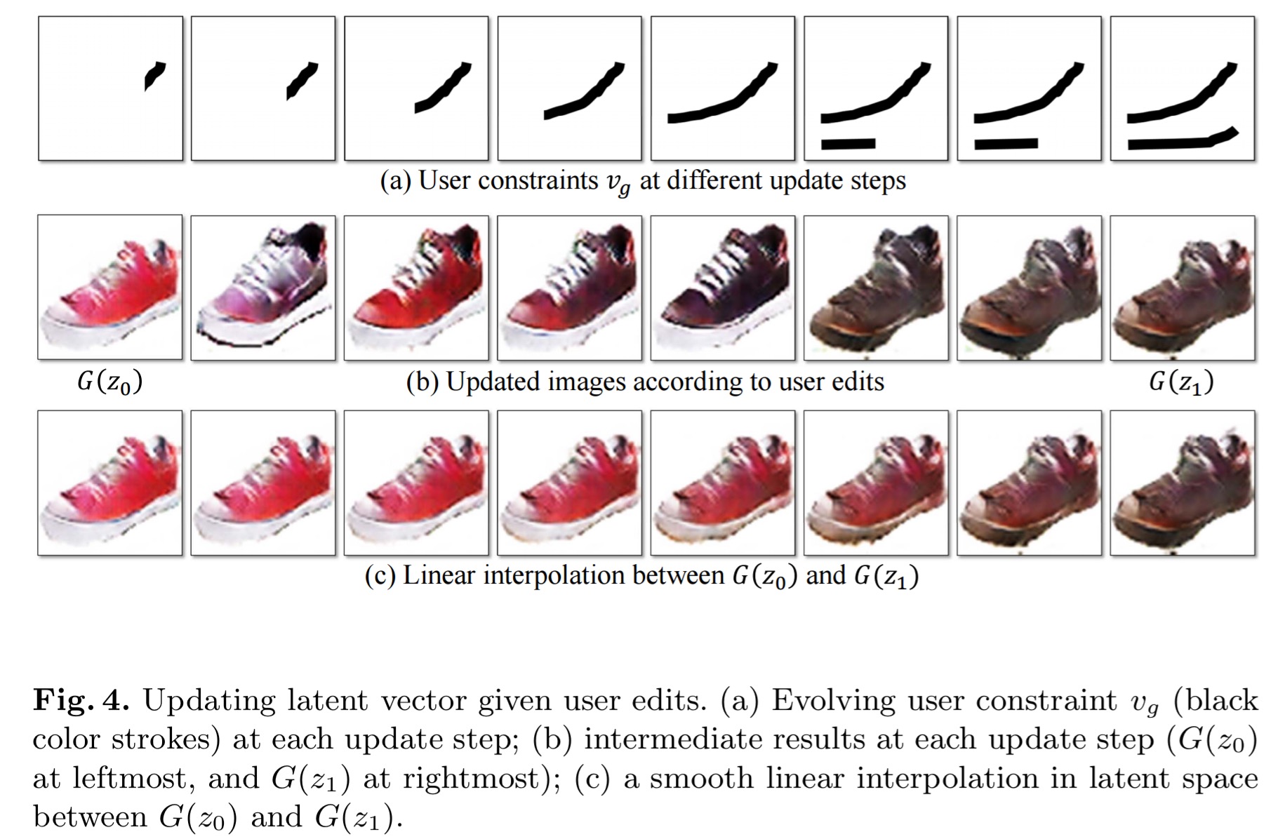
In the interactive tool, each update step takes about 50-100ms, working only on the mapped representation of the original image. When the user is done, the generated image captures roughly the desired change, but the quality is degraded as compared to the original image.
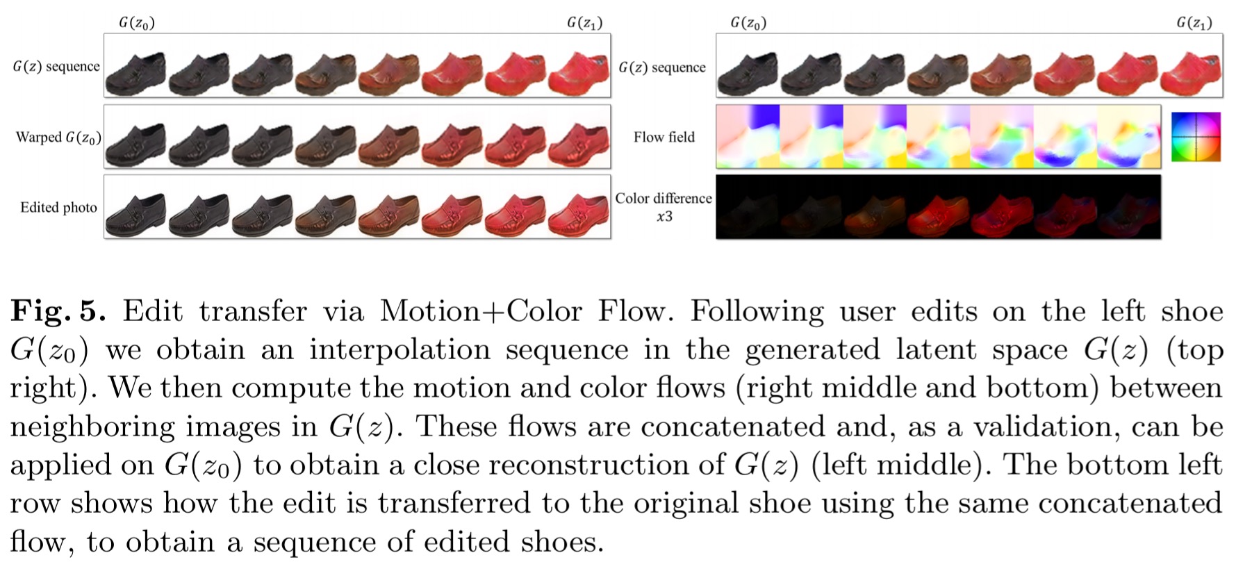
To address this issue, we develop a dense correspondence algorithm to estimate both the geometric and color changes induced by the editing process.
This motion and colour flow algorithm is used to estimate the colour and shape changes in the generated image sequence (as user editing progressed), and then transfer them back on top of the original photo to generate photo-realistic images.
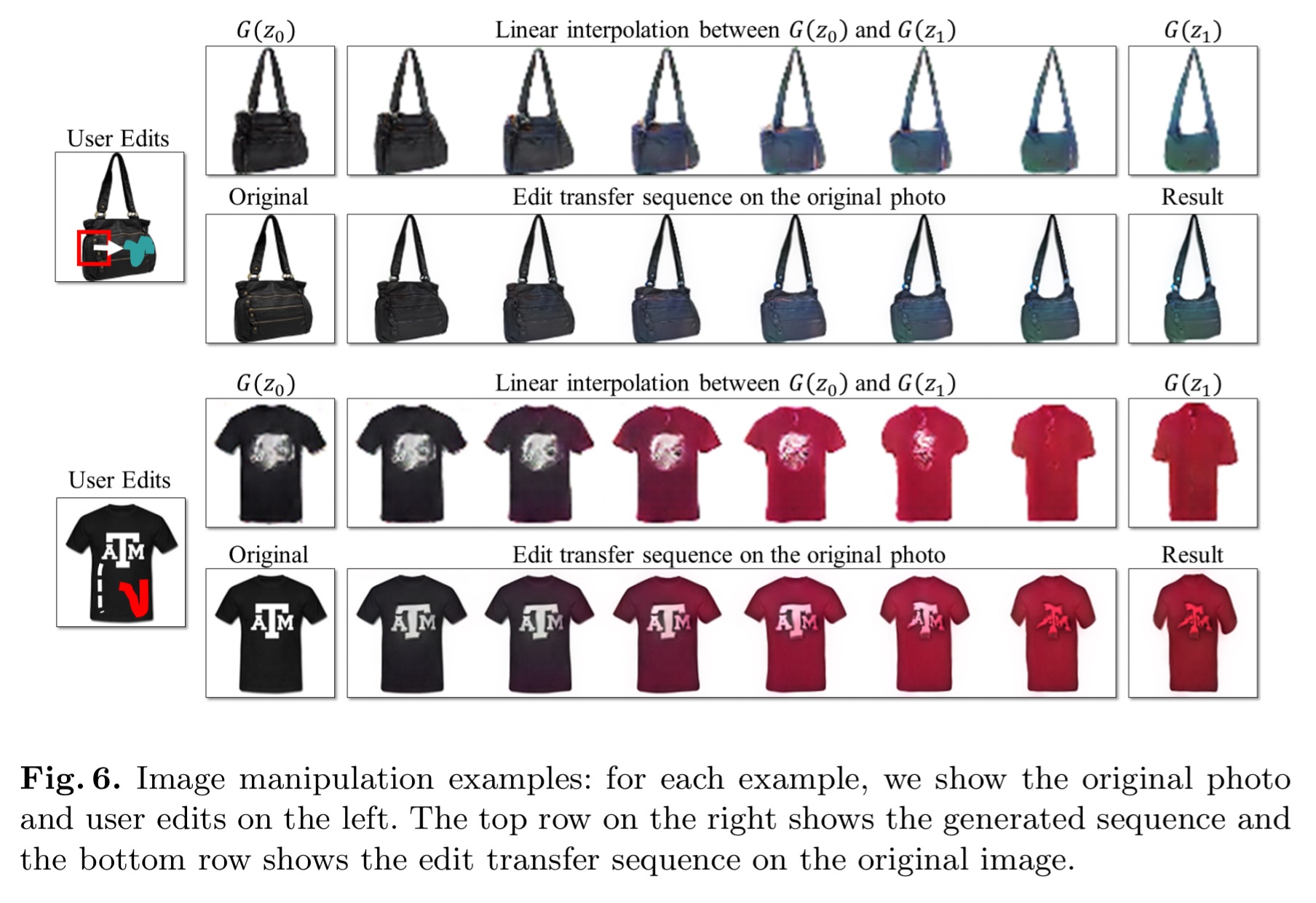
The user interface gives the user a colouring brush for changing the colour of regions, a sketching brush to outline shapes or add fine details, and a warping ‘brush’ for more explicit shape modifications.
Here are some results from user edits:
Transformations between two images also take place in the GAN-learned representation space and are mapped back in the same way:
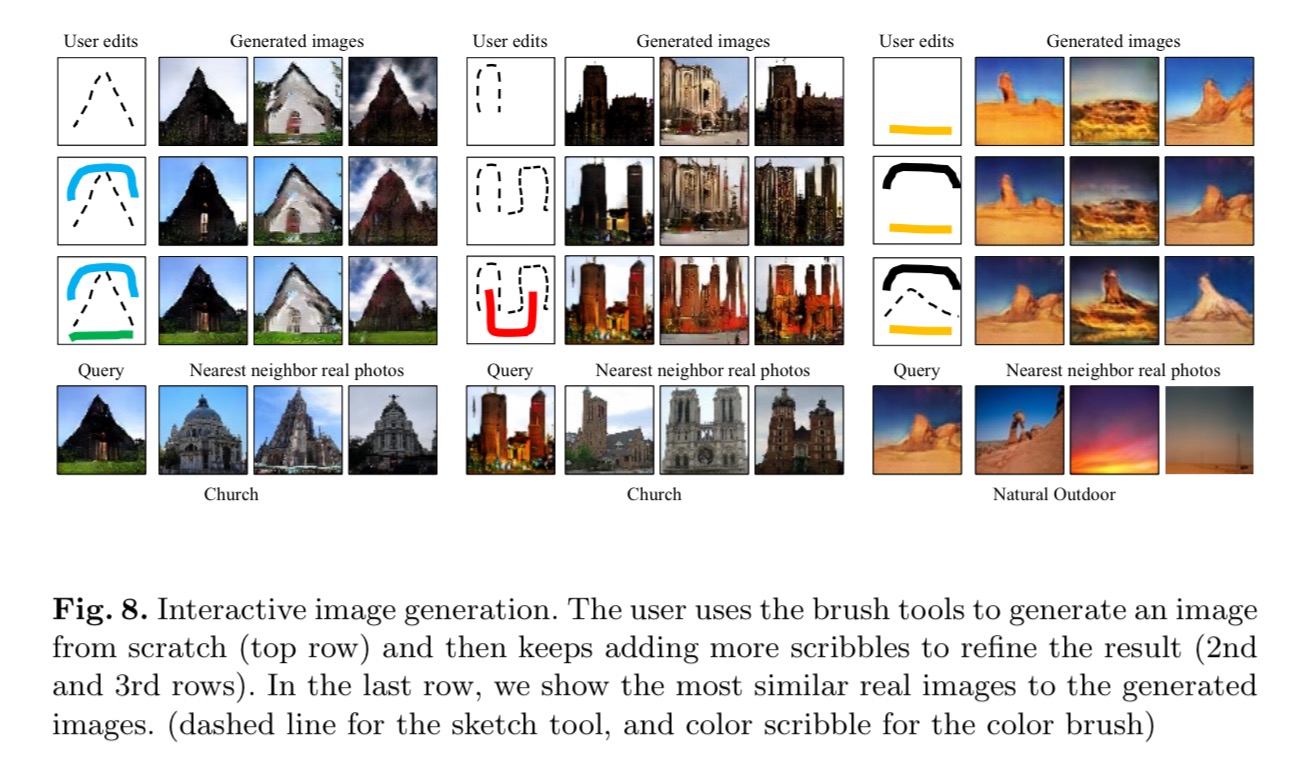
It’s also possible to use the brush tools to create an image from scratch, and then add more scribbles to refine the result. How good is this! :
WaveNet: a generative model for raw audio
Enough with the images already! What about generating sound? How about text-to-speech sound generation yielding state of the art performance? Hearing is believing, so check out these samples:
- WaveNet speaking in US English
- WaveNet trained without the accompanying text sequence, so that it has to make up what to say:
- WaveNet trained on classical piano music (just the audio, no score!) and left to its own devices to generate whatever it wants to:
(You can find more on the DeepMind blog at https://deepmind.com/blog/wavenet-generative-model-raw-audio/).
We show that WaveNets can generate raw speech signals with subjective naturalness never before reported in the field of text-to-speech (TTS), as assessed by human raters.
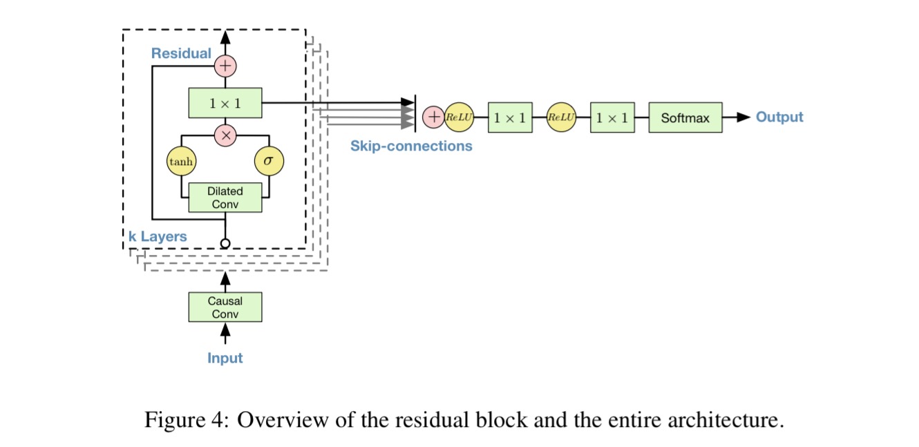
The architecture of WaveNet is inspired by PixelRNN (See “RNN models for image generation” from a couple of weeks ago). The foundation is very simple – take a waveform 


")
 = \prod_{t=1}^{T} p(x_t | x_1, ..., x_{t-1})")
This can be modelled by a stack of convolutional layers. “By using causal convolutions, we make sure the model cannot violate the ordering in which we model the data…” (the prediction at timestep t cannot depend on any of the future timestamps). This can be implemented by shifting the output of a normal convolution by one or more timesteps.
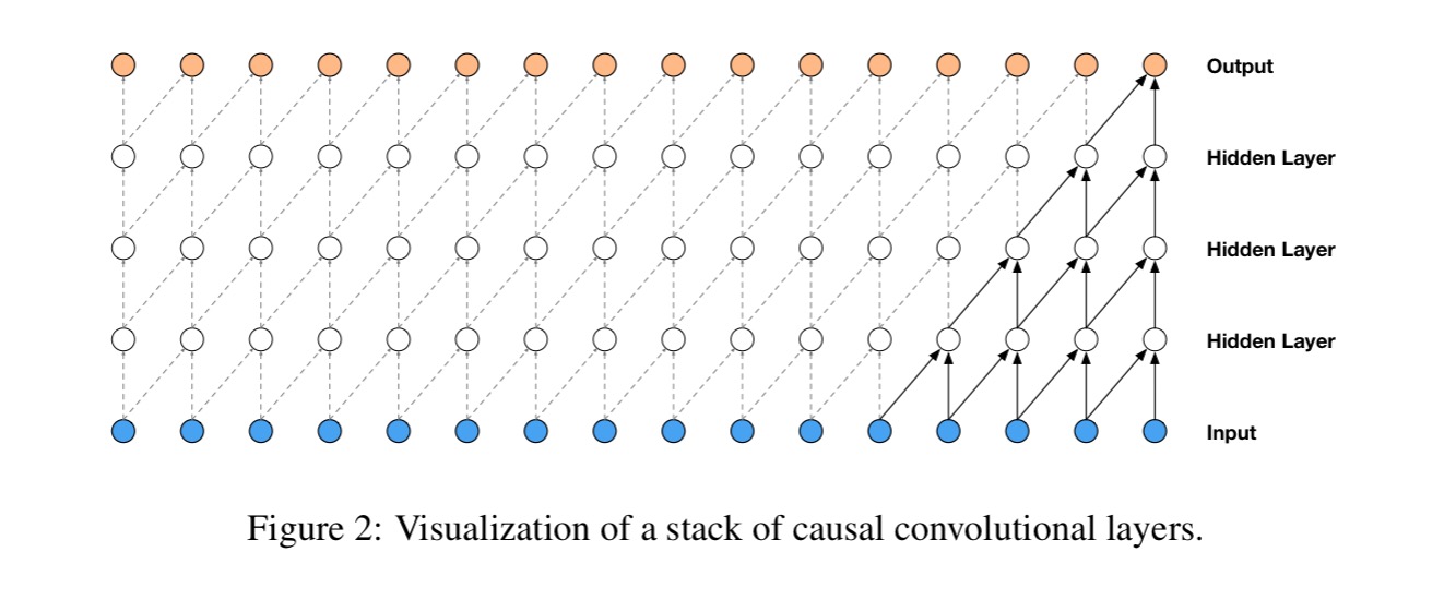
At training time, the conditional predictions for all timesteps can be made in parallel because all timesteps of ground truth x are known. When generating with the model, the predictions are sequential: after each sample is predicted, it is fed back into the network to predict the next sample.
Causal convolutions need lots of layers to increase their receptive field. WaveNet uses dilated convolutions to increase receptive fields by orders of magnitude, without greatly increasing computational cost.
A dilated convolution is a convolution where the filter is applied over an area large than its length by skipping input values with a certain step.
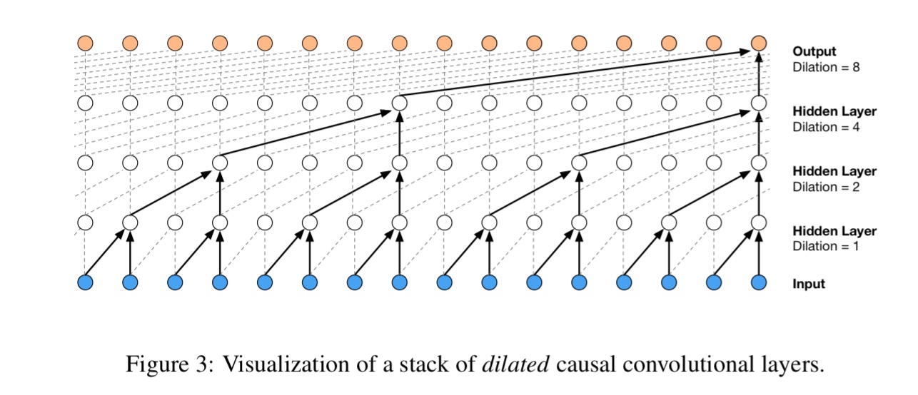
WaveNet uses dilation doubling in every layer up to a limit of 512, before repeating (1,2,4, …, 512, 1,2,4, …, 512, …).
A straight softmax output layer would need 65,356 probabilities per timestep to model all possible values for raw audio stored as a sequence of 16-bit integer values. The data is quantized to 256 possible values using a non-linear quantization scheme which was found to produce a significantly better reconstruction than a simple linear scheme:
 = sign(x_t) \frac{\ln(1 + \mu|x_t|)}{\ln(1 + \mu)}")
where 

 By conditioning the model on additional inputs, WaveNet can be guided to produce audio with the required characteristics (e.g., a certain speaker’s voice). For TTS, information about the text is fed as an extra input. > For the first experiment we looked at free-form speech generation (not conditioned on text). We used the English multi-speaker corpus from CSTR voice cloning toolkit (VCTK) (Yamagishi, 2012) and conditioned WaveNet only on the speaker. The conditioning was applied by feeding the speaker ID to the model in the form of a one-hot vector. The dataset consisted of 44 hours of data from 109 different speakers.
Since it wasn’t conditioned on text, the model generates made-up but human language-like words in a smooth way (see second audio clip at the top of this section). It can model speech from any of the speakers by conditioning it on the one-hot encoding – thus the model is powerful enough to capture the characteristics of all 109 speakers from the dataset in a single model.
The second experiment trained WaveNet on the same single-speaker speech databases that Google’s North American and Mandarin Chinese TTS systems are built on. WaveNet was conditioned on linguistic features derived from the input texts. In subjective paired comparison tests, WaveNet beat the best baselines:
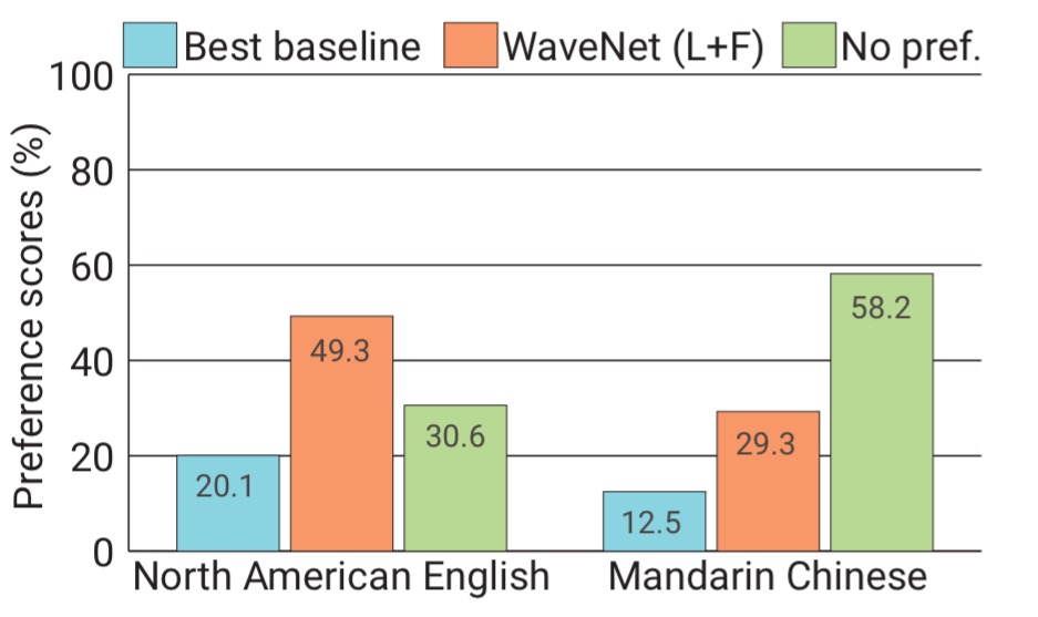
WaveNet also achieved the highest ever score in a mean opinion score test where users had to rate naturalness on a scale of 1-5 (scoring over 4 on average). (See the first speech sample at the top of this section).
The third set of experiments trained WaveNet on two music datasets (see the third speech sample at the top of this section). “…the samples were often harmonic and aesthetically pleasing, even when produced by unconditional models.”
From the WaveNet blog post on the DeepMind site:
WaveNets open up a lot of possibilities for TTS, music generation and audio modelling in general. The fact that directly generating timestep per timestep with deep neural networks works at all for 16kHz audio is really surprising, let alone that it outperforms state-of-the-art TTS systems. We are excited to see what we can do with them next.
Google’s neural machine translation system: bridging the gap between human and machine translation
Google’s Neural Machine Translation (GNMT) system is an end-to-end learning system for automated translation. Previous NMT systems suffered in one or more of three key areas: training and inference speed, coping with rare words, and sometimes failing to translate all of the words in a source sentence. GNMT is now in production at Google, having handsomely beaten the Phrase-Based Machine Translation (PBMT) system used in production at Google beforehand.
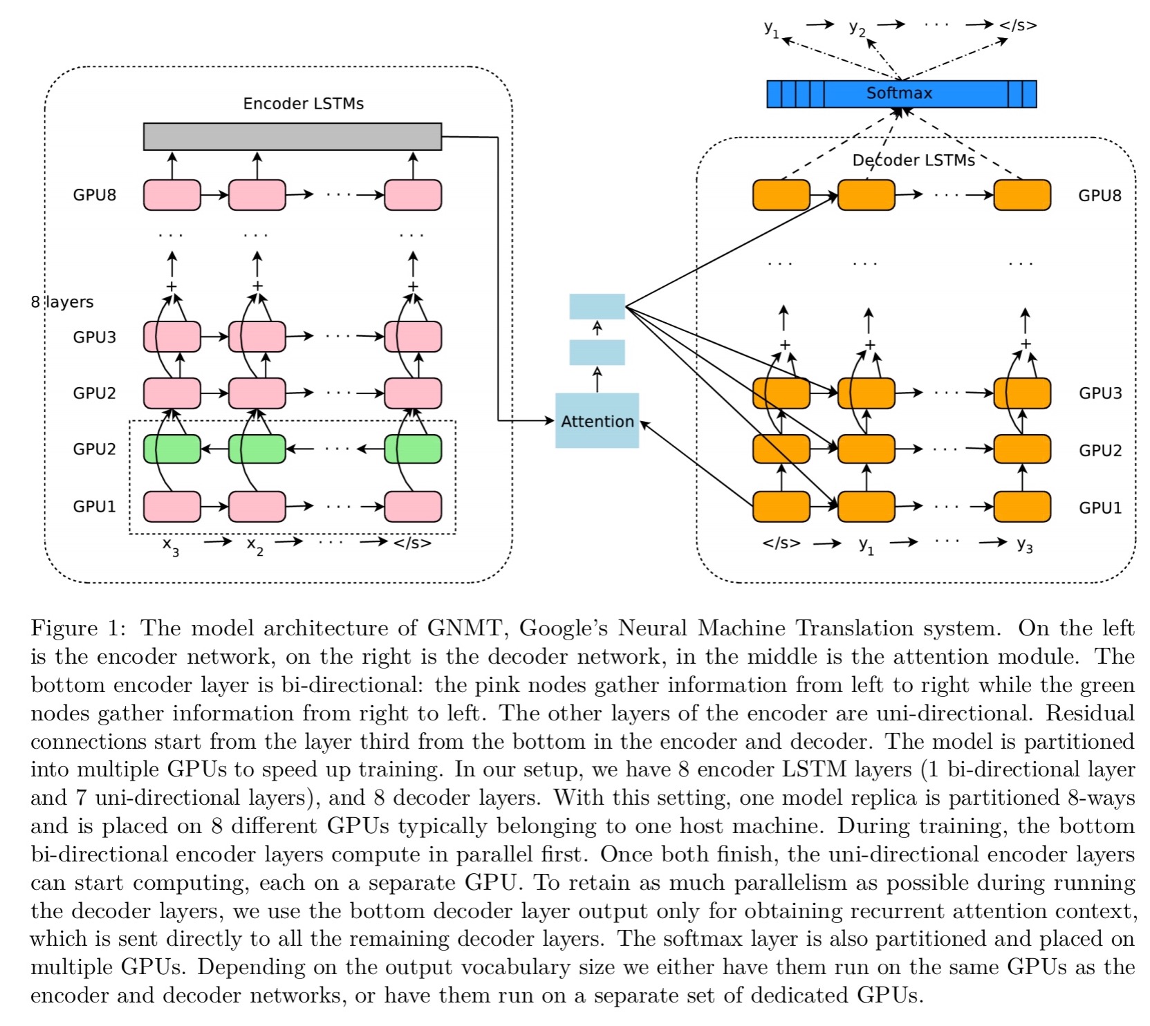
Understanding how it all fits together will draw upon many of the papers we’ve looked at so far. At the core it’s a sequence-to-sequence learning network with an encoder network, a decoder network, and an attention network.
The encoder transforms a source sentence into a list of vectors, one vector per input symbol. Given this list of vectors, the decoder produces one symbol at a time, until the special end-of-sentence symbol (EOS) is produced. The encoder and decoder are connected through an attention module which allows the decoder to focus on different regions of the source sentence during the course of decoding.
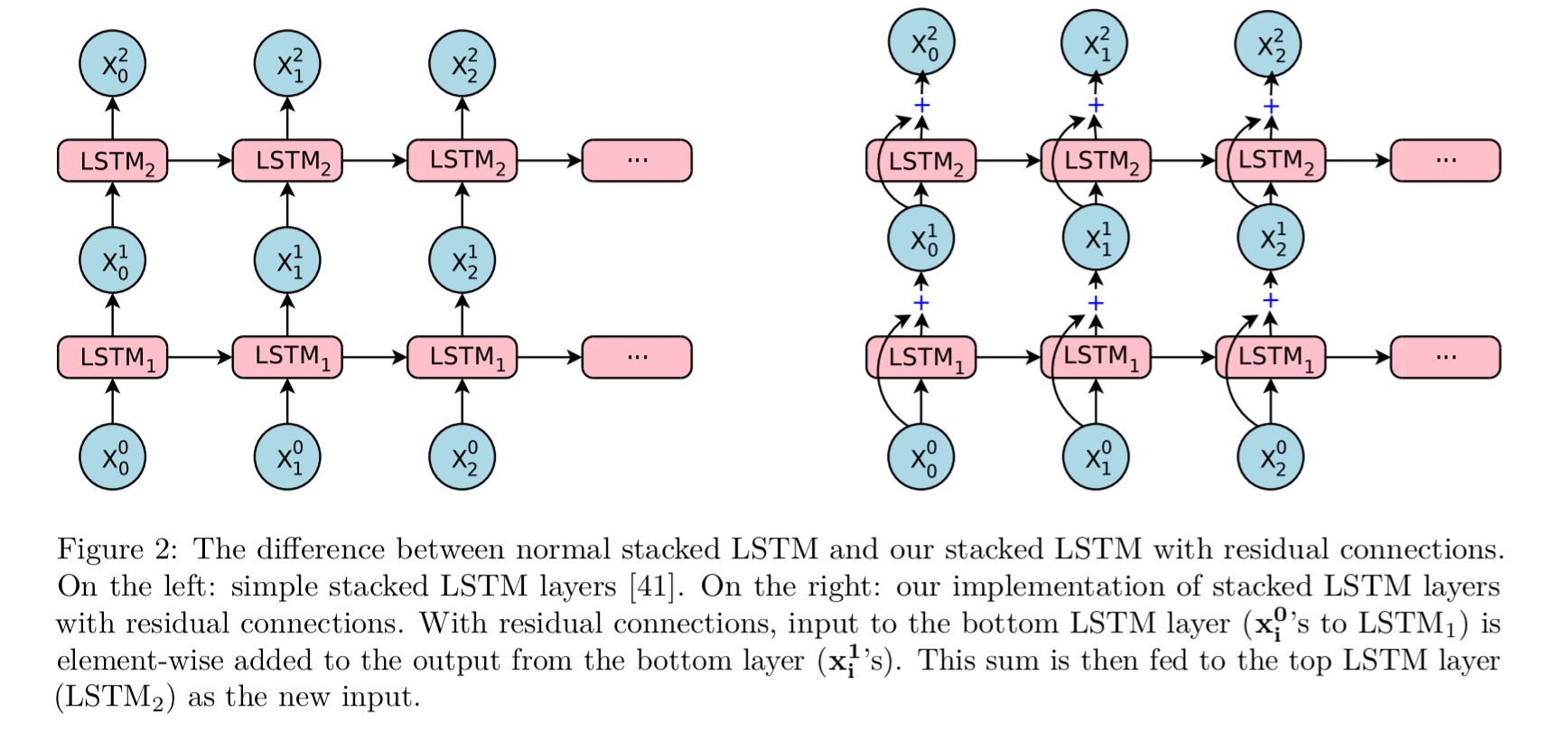
The decoder is a combination of an RNN network and a softmax layer. Deeper models give better accuracy, but the team found that LSTM layers worked well up to 4 layers, barely with 6 layers, and very poorly beyond 8 layers. What to do? We learned the answer earlier this week, add residual connections:
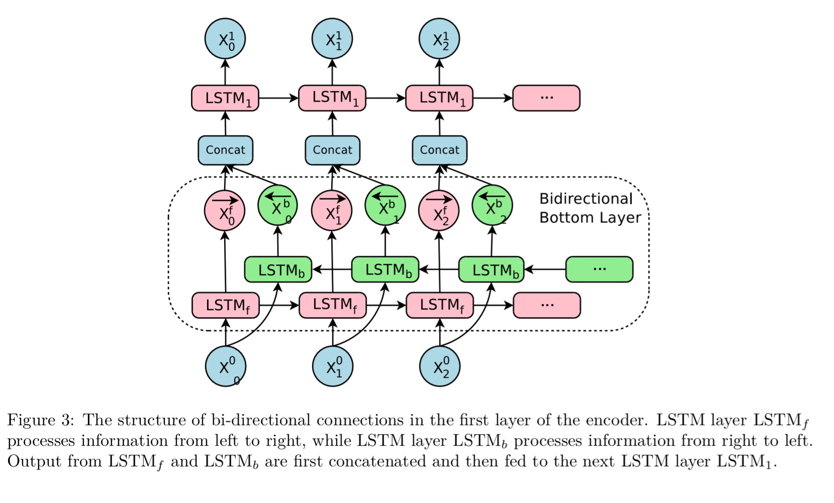
Since in translation words in the source sentence may appear anywhere in the output sentence, the encoder network uses a bi-directional RNN for the encoder. Only the bottom layer is bi-direction – one LSTM layer processes the sentence left-to-right, while its twin processes the sentence right-to-left.
The encoder and decoder networks are placed on multiple GPUs, with each layer running on a different GPU. As well as using multiple GPUs, to get inference time down quantized inference involving reduce precision arithmetic is also used.
One of the main challenges in deploying our Neural Machine Translation model to our interactive production translation service is that it is computationally intensive at inference, making low latency translation difficult, and high volume deployment computationally expensive. Quantized inference using reduced precision arithmetic is one technique that can significantly reduce the cost of inference for these models, often providing efficiency improvements on the same computational devices.
The model is trained using full-precision floats, it is only for production inference that approximation is used. Here are the decoding times for 6003 English-French sentences across CPU, GPU, and Google’s Tensor Processing Unit (TPU) respectively:
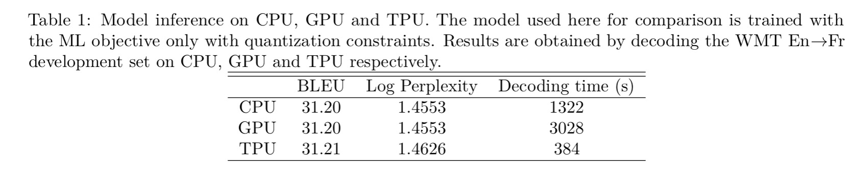
Firstly, note that the TPU beats the CPU and GPU hands-down. The CPU beats the GPU because “our current decoder implementation is not fully utilizing the computation capacities that a GPU can theoretically offer during inference.”
Dealing with out of vocabulary words
Neural Machine Translation models often operate with fixed word vocabularies even though translation is fundamentally an open vocabulary problem (names, numbers, dates etc.)… Our most successful approach […] adopts the wordpiece model (WPM) implementation initially developed to solve a Japanese/Korean segmentation problem for the Google speech recognition system. This approach is completely data-driven and guaranteed to generate a deterministic segmentation for any possible sequence of characters.
For example, “Jet makers feud over seat width with big orders at stake” turns into the word pieces: “_J et _makers _fe ud _over _seat _width _with _big _orders _at _stake.” The words ‘Jet’ and ‘feud’ are both broken into two word pieces.
Given a training corpus and a number of desired tokens D, the optimization problem is to select D wordpieces such that the resulting corpus is minimal in the number of wordpieces when segmented according to the chosen wordpiece model.
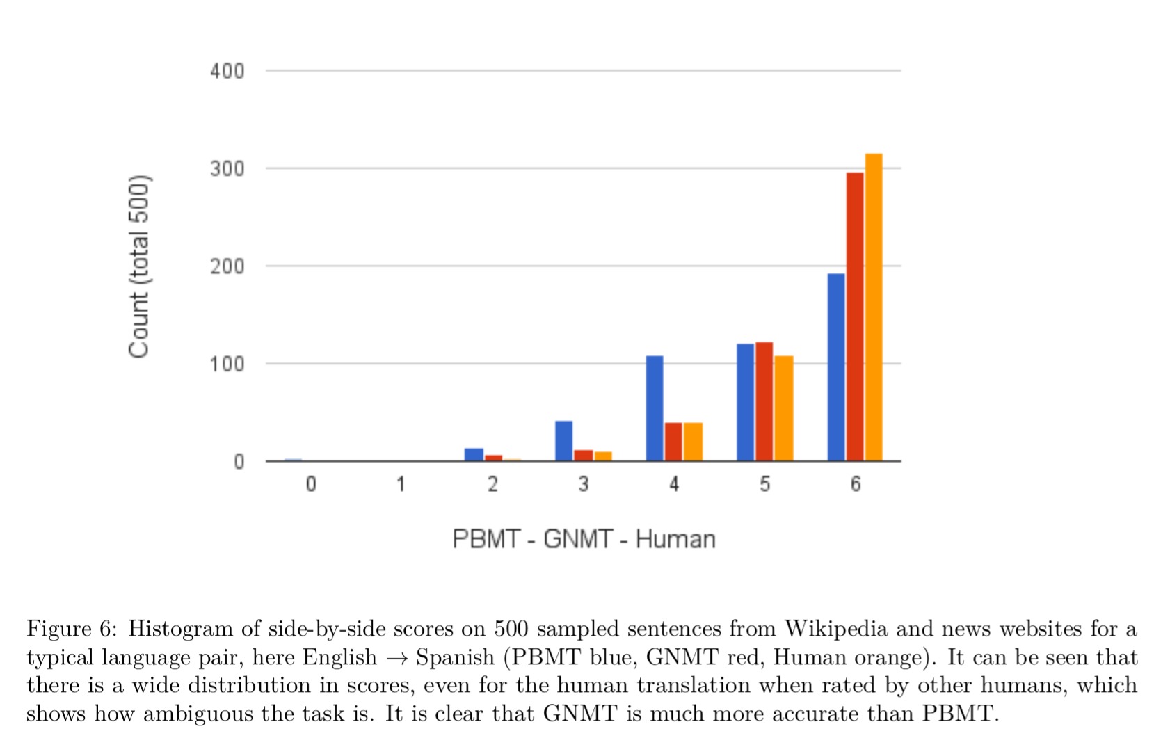
Overall model performance.
The following chart shows side-by-side scores for translations made by the previous production system (PBMT), the new GNMT system, and humans fluent in both languages.
Side-by-side scores range from 0 to 6, with a score of 0 meaning “completely nonsense translation”, and a score of 6 meaning “perfect translation: the meaning of the translation is completely consistent with the source, and the grammar is correct”. A translation is given a score of 4 if “the sentence retains most of the meaning of the source sentence, but may have some grammar mistakes”, and a translation is given a score of 2 if “the sentence preserves some of the meaning of the source sentence but misses significant parts”. These scores are generated by human raters who are fluent in both languages and hence often capture translation quality better than BLEU scores.