Today it’s the second tranche of papers from the convolutional neural nets section of the ‘top 100 awesome deep learning papers‘ list:
- Return of the devil in the details: delving deep into convolutional nets, Chatfield et al., 2014
- Spatial pyramid pooling in deep convolutional networks for visual recognition, He et al., 2014
- Very deep convolutional networks for large-scale image recognition, Simonyan & Zisserman, 2014
- Going deeper with convolutions, Szegedy, 2015
Return of the devil in the details: delving deep into convolutional nets
This is a very nice study. CNNs had been beating handcrafted features in image recognition tasks, but it was hard to pick apart what really accounted for the differences (and indeed, the differences between different CNN models too) since comparisons across all of them were not done on a shared common basis. For example, we’ve seen augmentation typically used with CNN training – how much of the difference between IVF (the Improved Fisher Vector hand-engineered feature representation) and CNNs is attributed to augmentation, and not the image representation used? So Chatfield et al. studied IFV shallow representation, three different CNN-based deep representations, and deep representations with pre-training and then fine-tuning on the target dataset. For all of the studies, the same task (PASCAL VOC classification) was used. The three different CNN representations are denoted CNN-F (Fast) – based on Krizhevksy’s architecture; CNN-M (Medium) – using a decreased stride and smaller receptive field of the first convolutional layer; and CNN-S (Slow) based on the ‘accurate’ network from OverFeat.
Key findings:
- Augmentation improves performance by ~3% for both IFV and CNNs. (Or to put it another way, the use of augmentation accounts for 3% of the advantage attributed to deep methods). Flipping on its own helps only marginally, but flipping combined with cropping works well.
- Both IFV and CNNs are affected by adding or subtracting colour information. Retraining CNNs after converting images to grayscale results in about a 3% performance drop.
- CNN based methods still outperform shallow encodings, even accounting for augmentation improvements etc., by a large approximately 10% margin.
- CNN-M and CNN-S both outperform CNN-Fast by 2-3%. CNN-M is about 25% faster than CNN-S.
- Retraining the CNNs so that the final layer was of lower dimensionality resulted in a marginal performance boost.
- Fine-tuning makes a significant difference, improving results by about 2.7%.
In this paper we presented a rigorous empirical evaluation of CNN-based methods for image classification, along with a comparison with more traditional shallow feature encoding methods. We have demonstrated that the performance of shallow representations can be significantly improved by adopting data augmentation, typically used in deep learning. In spite of this improvement, deep architectures still outperform the shallow methods by a large margin. We have shown that the performance of deep representations on the ILSVRC dataset is a good indicator of their performance on other datasets, and that fine-tuning can further improve on already very strong results achieved using the combination of deep representations and a linear SVM.
Spatial pyramid pooling in deep convolutional networks for visual recognition
The CNN architectures we’ve looked at so far have a series of convolutional layers (5 is popular) followed by fully connected layers and an N-way softmax output. One consequence of this is that they can only work with images of fixed size (e.g 224 x 224). Why? The sliding windows used in the convolutional layers can actually cope with any image size, but the fully-connected layers have a fixed sized input by construction. It is the point at which we transition from the convolution layers to the fully-connected layers therefore that imposes the size restriction. As a result images are often cropped or warped to fit the size requirements of the network, which is far from ideal.
Spatial pyramid pooling (SPP) adds a new layer between the convolutional layers and the fully-connected layers. Its job is to map any size input down to a fixed size output. The ideal of spatial pyramid pooling, also know as spacial pyramid matching or just ‘multi-level pooling’ pre-existed in computer vision, but had not been applied in the context of CNNs.
SPP works by dividing the feature maps output by the last convolutional layer into a number of spatial bins with sizes proportional to the image size, so the number of bins is fixed regardless of the image size. Bins are captured at different levels of granularity – for example, one layer of 16 bins dividing the image into a 4×4 grid, another layer of 4 bins dividing the image into a 2×2 grid, and a final layer comprising the whole image. In each spatial bin, the responses of each filter are simply pooled using max pooling.
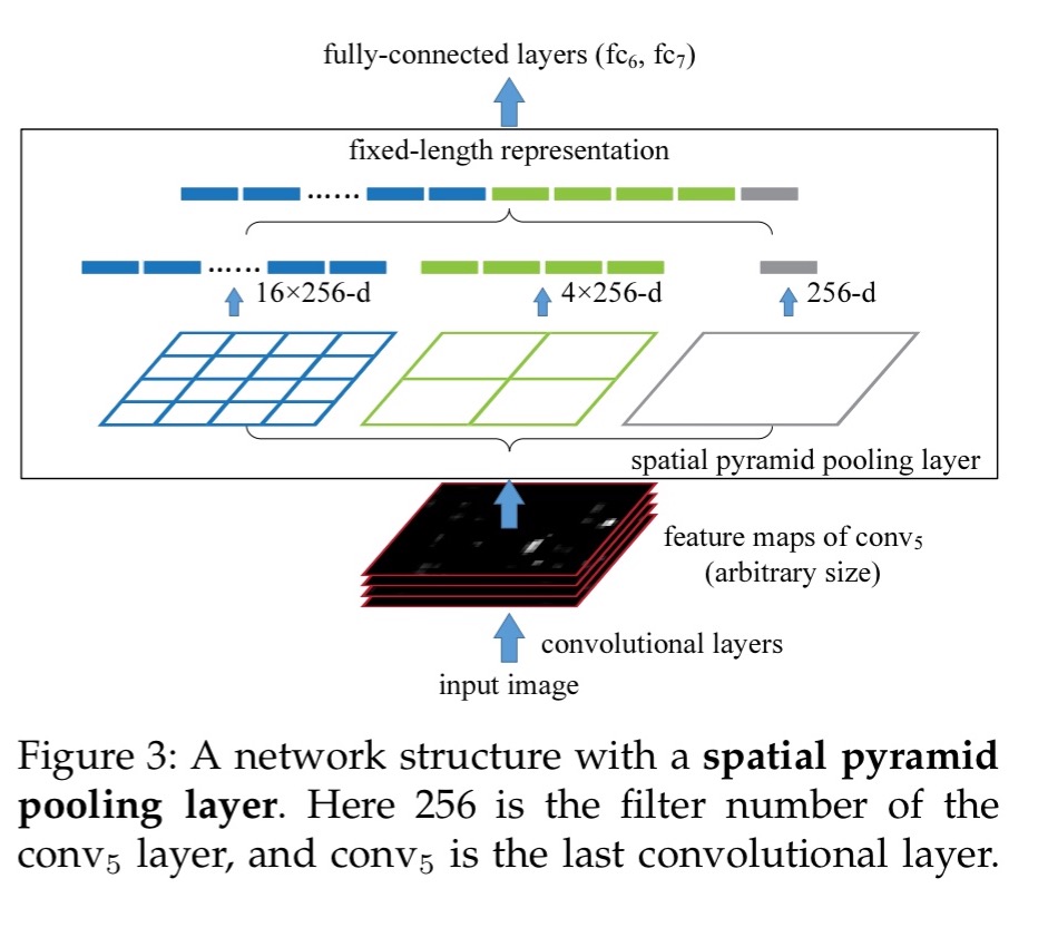
Since the number of bins is known, we can just concatenate the SPP outputs to give a fixed length representation (see the figure above).
This not only allows arbitrary aspect ratios, but also allows arbitrary scales… When the input image is at different scales, the network will extract features at different scales. Interestingly, the coarsest pyramid level has a single bin that covers the entire image. This is in fact a “global pooling” operation, which is also investigated in several concurrent works.
An SPP layer added to four different networks architects, including AlexNet (Krizhevsky et al.) and OverFeat improved the accuracy of all of them. “The gain of multi-level pooling is not simply due to more parameters, rather it is because the multi-level pooling is robust to the variance in object deformations and spatial layout.”
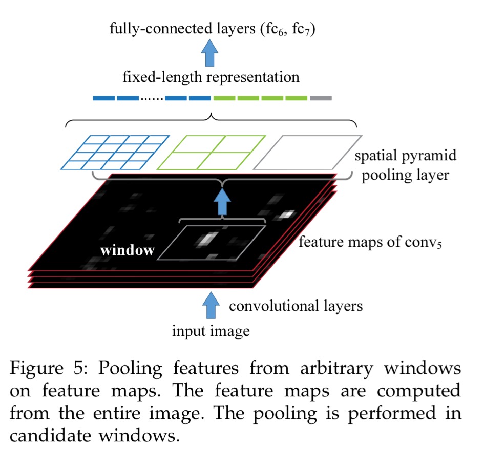
The SPP technique can also be used for detection. The state-of-the-art (as of time of publication) R-CNN method runs feature extraction on each of 2000 candidate windows extracted from an input image. This is expensive and slow. An SPP-net used for object detection extracts feature maps only once (possible at multiple scales). Then just the spatial pyramid pooling piece is run once for each candidate window. This turns out to give comparable results, but with running times 38x-102x faster depending on the number of scales.
Very deep convolutional networks for large-scale image recognition
We’ve now seen the ConvNet architecture and some variations exploring what happens with different window sizes and strides, and training and testing at multiple scales. In this paper Simonyan and Zisserman hold all those variables fixed, and explore what effect the depth of the network has on classification accuracy.
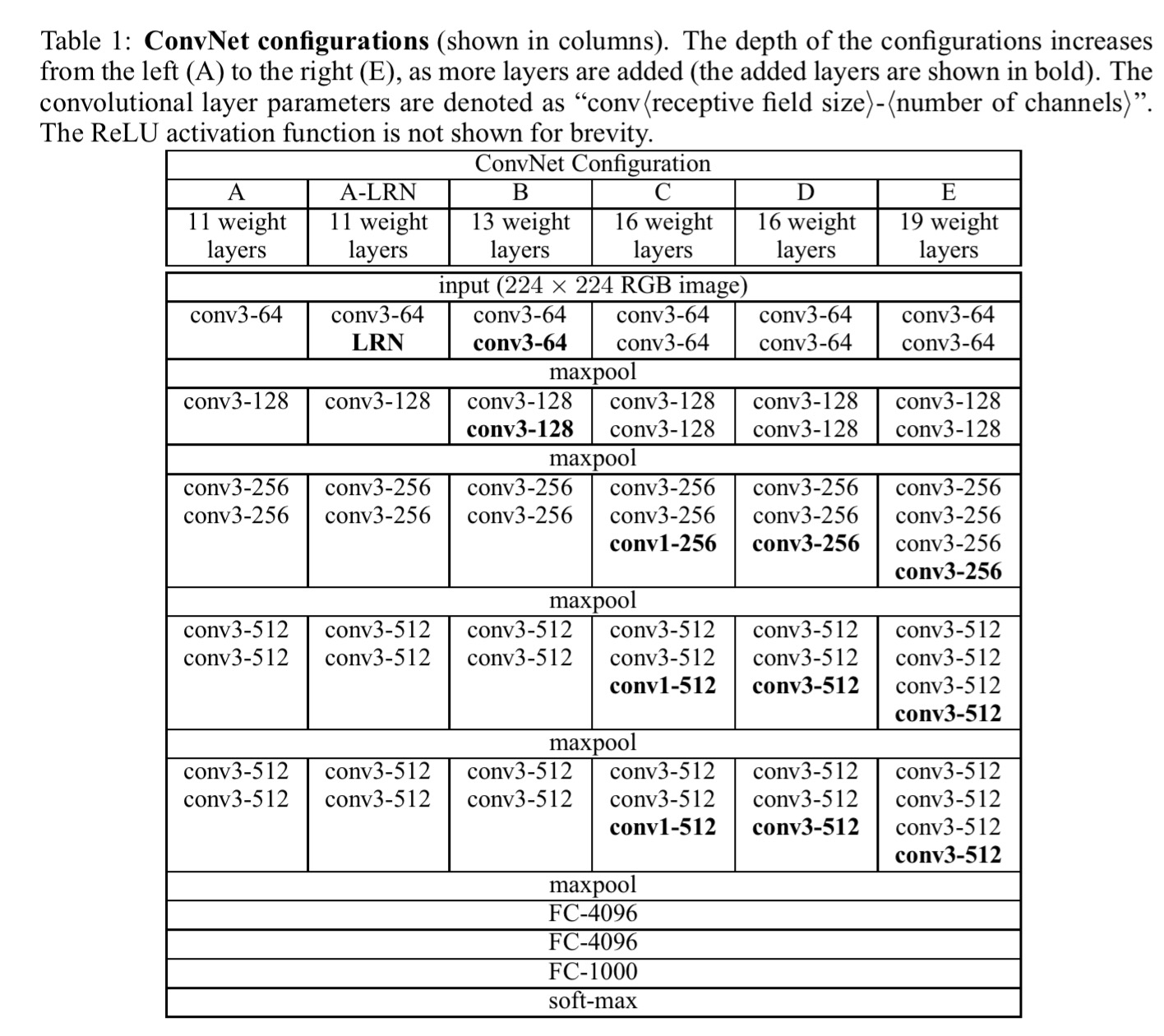
The basic setup is a fixed-size 224 x 224 RGB input image with mean pixel value (computed over the training set) subtracted from each pixel. A stack of convolutional layers (with varying depth in each of the experiments) uses filters with a 3×3 receptive field, and in one configuration a layer is added with a 1×1 field (which can be seen as a linear transformation of the input channels, followed by non-linearity). The stride is fixed at 1 pixel. Spatial pooling is carried out by five max-pooling layers interleaved with the convolutional layers. This stack is then feed into three fully-connected layers and a final soft-max layer. The hidden layers all use ReLU activation.
Given this basic structure, the actual networks evaluated are shown in the table below (note that only one of them uses local response normalisation – LRN):
Here’s what the authors find:
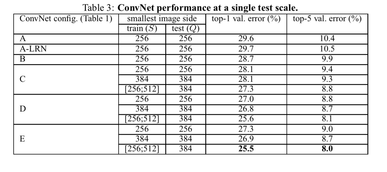
Firstly, local response normalisation did not improve accuracy (A-LRN vs A), but adds to training time, so it is not employed in the deeper architectures. Secondly, classification error decreases with increased ConvNet depth (up to 19 layers in configuration E).
The error rate of our architecture saturates when the depth reaches 19 layers, but even deeper models might be beneficial for larger datasets. We also compared the net B with a shallow net with five 5 × 5 conv. layers, which was derived from B by replacing each pair of 3 × 3 conv. layers with a single 5 × 5 conv. layer (which has the same receptive field as explained in Sect. 2.3). The top-1 error of the shallow net was measured to be 7% higher than that of B (on a center crop), which confirms that a deep net with small filters outperforms a shallow net with larger filters.
The results above were achieved when training at a single scale. Even better results were achieved by adding scale jittering at training time (lightly rescaled versions of the original image).
Going deeper with convolutions
So now things start to get really deep! This is the paper that introduced the ‘Inception’ network architecture, and a particular instantiation of it called ‘GoogLeNet’ which achieved a new state of the art in the 2014 ISLVRC (ImageNet) competition. GoogLeNet is 22 layers deep, and has a pretty daunting overall structure, which I thought I’d just include here in its full glory!
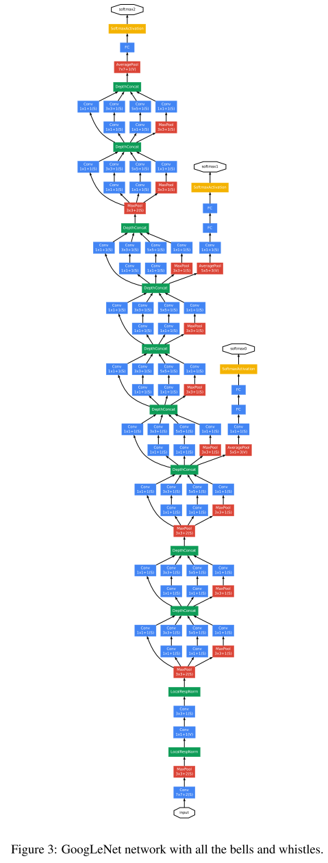
Despite the intimidating looking structure, GoogLeNet actually uses 12x fewer parameters than the winning Krizhevsky ConvNet of two years prior. At the same time, it is significantly more accurate. Efficiency in terms of power and memory use was an explicit design goal of the Inception architecture:
It is noteworthy that the considerations leading to the design of the deep architecture presented in this paper included this factor [efficiency] rather than having a sheer fixation on accuracy numbers. For most of the experiments, the models were designed to keep a computational budget of 1.5 billion multiply-adds at inference time, so that they do not end up to be a purely academic curiosity, but could be put to real world us, even on large datasets, at a reasonable cost.
You can always make your network ‘bigger’ (both in terms of number of layers – depth, as well as the number of units in each layer – width), and in principle this leads to higher quality models. However, bigger networks have many more parameters making them prone to overfitting. To avoid this you need much more training data. They also require much more computational resource to train. “For example, in a deep vision network if two convolutional layers are chained, any uniform increase in the number of their filters results in a quadratic increase in computation.”
One way to counteract this is to introduce sparsity. Arora et al., in “Provable bounds for learning some deep representations” showed that if the probability distribution of the dataset is representable by a large, very sparse deep neural network, then the optimal network technology can be constructed layer after layer by analyzing the correlation statistics of the preceding layer activations and clustering neurons with highly correlated outputs.
Unfortunately, today’s computing infrastructures are very inefficient when it comes to numerical calculation on non-uniform sparse data structures.
Is there any hope for an architecture that makes use of filter-level sparsity, as suggested by the theory, but exploits current hardware by utilizing computations on dense matrices? The Inception architecture started out as an exploration of this goal.
The main idea of the Inception architecture is to consider how an optimal local sparse structure of a convolutional vision network can be approximated and covered by readily available dense components.
Given the layer-by-layer construction approach, this means we just have to find the optimal layer structure, and then stack it. The basic structure of an Inception layer looks like this:
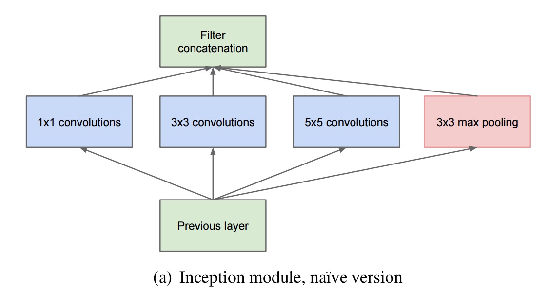
The 1×1 convolutions detect correlated units in local regions, and the larger (3×3 and 5×5) convolutions detect the (smaller number) of more spatially spread out clusters. Since pooling has been shown to have a beneficial effect, a pooling path in each stage is added for good luck too.
The problem with the structure as shown above though, is that it is prohibitively expensive!
While this architecture might cover the optimal sparse structure, it would do it very inefficiently, leading to a computational blow up within a few stages.
The solution is to reduce the network dimensions using 1×1 convolutions on all the 3×3 and 5×5 pathways. “Beside being used as reductions, they also include the use of rectified linear activation making them dual purpose.” This gives a final structure for an Inception layer that looks like this:
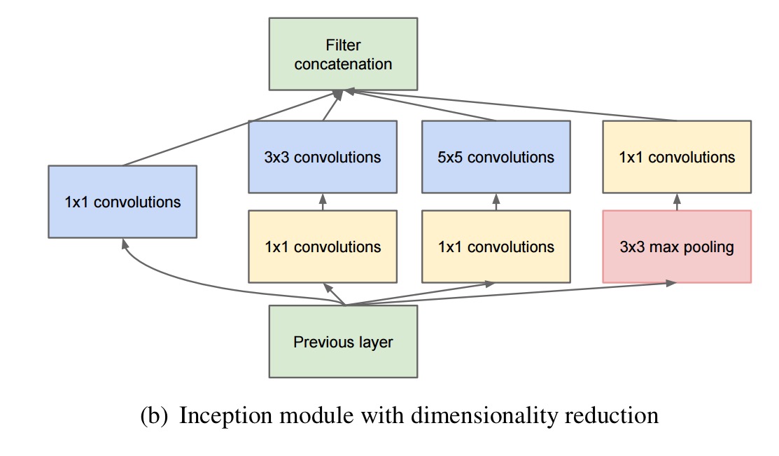
In general, an Inception network is a network consisting of modules of the above type stacked upon each other, with occasional max-pooling layers with stride 2 to halve the resolution of the grid.
You can see these layers stacked on top of each other in the GoogLeNet model. That network is 22 layers deep (27 if the pooling layers are also counted). The overall number of building blocks used for the construction of the network is about 100! Propagating gradients all the way back through so many layers is a challenge. We know that shallower networks still have strong discriminative performance, and this fact was exploited by adding auxiliary classifiers connected to intermediate layers (yellow boxes in the overall network diagram at the start of this section)…
… These classifiers take the form of smaller convolutional networks put on top of the output of the Inception (4a) and (4d) modules. During training, their loss gets added to the total loss of the network with a discount weight (the losses of the auxiliary classifiers were weighted by 0.3). At inference time, these auxiliary networks are discarded.