Shasta: Interactive Reporting At Scale Manoharan et al., SIGMOD 2016
You have vast database schemas with hundreds of tables, applications that need to combine OLTP and OLAP functionality, queries that may join 50 or more tables across disparate data sources, oh, and the user is waiting, so you’d better deliver the results online with low latency.
It sounds like a recipe for disaster, yet this is exactly the situation that Google faced with many of its business systems, especially it seems with their advertising campaign management system. Business logic and data transformation logic was becoming tangled bottlenecking development, queries were way too large to be expressed gracefully in SQL (especially when considering the dynamic aspects), and traditional techniques to speed up queries such as maintaining materialized views either increased the cost of writes too much, or gave unacceptably stale data.
Shasta is the system that Google developed in response to these challenges. At the front-end, Shasta enables developers to define views and express queries in RVL, a new Relational View Language. Shasta translates RVL queries into SQL queries before passing them onto F1. Shasta does not rely on pre-computation, instead a number of optimisations in the underlying data infrastructure enable it to achieve the desired latency targets.
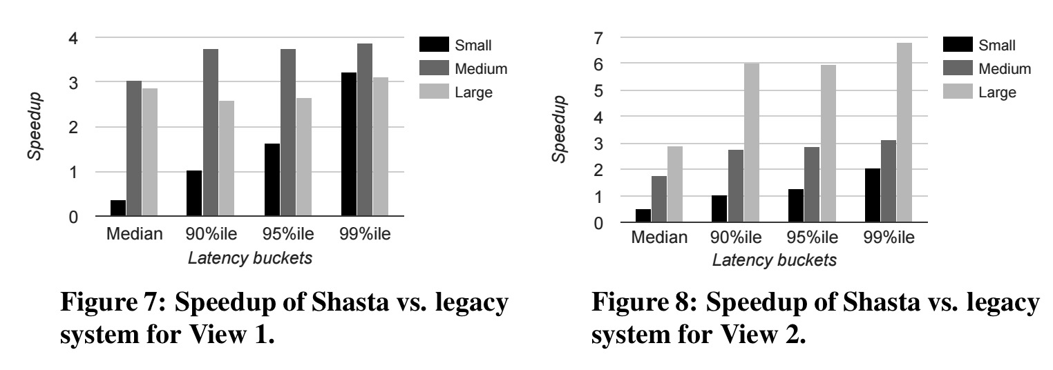
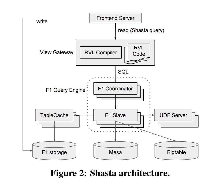
Using Shasta, an ‘important advertiser-facing application’ was reduced from 130K lines of C++ view definitions to about 30K lines of RVL and 23K lines of C++ UDF code. Using the techniques we’ll dive into shortly, Shasa also performed 2.5-7.5x faster on large queries, and 2-4x faster on medium queries compared to the old system. (Small queries are actually slower in Shasta, since the overhead of all the RVL parsing machinery is not paid back sufficiently).
The key requirements for Shasta are:
- Cope with diverse underlying data stores (which is achieved by using F1s ability to scan external tables)
- Handle complex view computations involving many tens of tables
- Reflect data updates immediately
- Low latency responses – Shasta queries are on the critical path for rendering pages in user-facing apps with sub-second latency targets.
- Support parameterized view definitions for maximum reuse
- Enable developers to easily reason about and modify views.
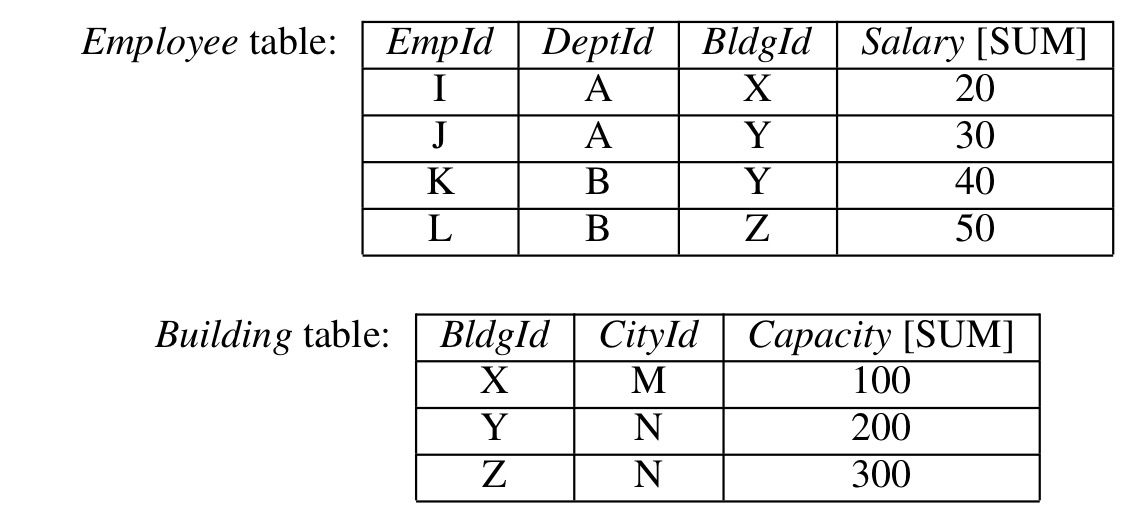
The big picture architecture looks like this:
An application generates a query specifying a view name, columns of interest, and any view parameters as well as an optional timestamp telling Shasta to use an F1 snapshot consistent with that timestamp. The view gateway invokes the RVL compiler with the given parameter bindings, which generates a (potentially large) SQL string. This is then executed by the F1 query engine. TableCache is an in-memory cache that accelerates access to F1 storage.
TableCache acts as an extra layer of caching between the F1 query engine and F1 storage backed by Spanner. It can be compared to the usage of buffer pools in traditional database architectures since the goal is to exploit database access patterns to accelerate I/O. However, TableCache is read-only, which allows the design to be optimized for the read path without sacrificing write performance. In particular, TableCache uses fine-grained sharding to perform many small reads in parallel, and trans actional writes become more expensive with higher degrees of parallelism. Also, TableCache provides a higher-level abstraction than traditional block-based caches, where data from a table is accessed based on root ID and timestamp.
There are a number of enhancements to F1 that help to make Shasta queries efficient, TableCache being one of the more significant (see §5 and §6 for details) . Most interesting from my perspective though is the rationale for introducing a new query language, RVL, and what it looks like.
RVL: A relational view language
The syntax of RVL is similar to SQL, but with semantic differences oriented towards OLAP applications. The most important of these is support for automatic aggregation of data when columns are projected, based on information contained in the schema itself. The query language is embedded in higher-level constructs called view templates . These support abstraction through parameterisation, and composition of templates and queries to allow a view’s implementation to be factored into manageable and reusable pieces.
If the metadata for a column specifies an optional implicit aggregation function then it is treated as as aggregatable column. Otherwise it is a grouping column.
… the grouping columns always form a unique key for a relation in RVL, and the aggregatable columns represent measures associated with values of the unique key.
Exploiting these mechanisms, RVL queries may be much more succinct than their SQL counterparts, and also afford additional optimisation opportunities over and above those that the query optimiser in F1 can perform.
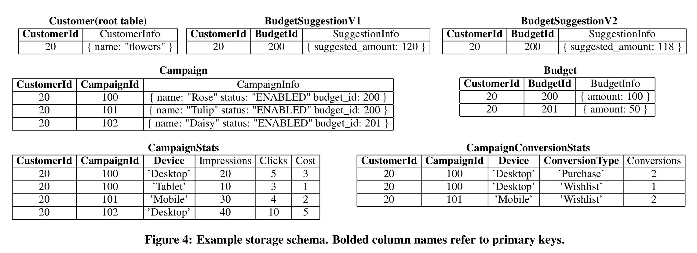
Consider the following two tables:
We can write an RVL query to join Employee and Building as follows:
Q0 = SELECT *
     FROM Employee LEFT JOIN Building USING (BldgId);
And then reuse that building block to find the total salary for each department:
Q1 = SELECT DeptId, Salary FROM Q0;
Since Salary has an aggregate function it will automatically be summed. Since DeptId doesn’t it will automatically be used as a grouping column. Of course Q1 doesn’t actually need any data at all from the Building table, and the RVL compiler is smart enough to do join pruning resulting in the following generated SQL:
SELECT DeptId, SUM(Salary) FROM Employee
 GROUP BY DeptId
We could also reuse Q0 in another query that does need information from both tables:
Q2 = SELECT CityId, Salary, Capacity FROM Q0;
Now we can start to see how much easier to read this is than the corresponding generated SQL:
SELECT CityId, SUM(Salary) AS Salary,
       SUM(Capacity) AS Capacity
FROM
   (SELECT BldgId, SUM(Salary) AS Salary
    FROM Employee GROUP BY BldgId)
   LEFT JOIN Building USING (BldgId)
GROUP BY CityId;
The value of RVL can be seen by comparing Q1 and Q2 to the corresponding SQL representations. In RVL, we can define a single subquery Q0 such that Q1 and Q2 can be expressed as simple projections over Q0. In contrast, the SQL representations of Q1 and Q2 have drastically different structure. RVL also makes it easy to derive meaningful aggregate values from Q0 for many other combinations of grouping columns.
Real Shasta queries tend to be much more complex, requiring dozens of tables to be joined – RVL makes formulating such queries much simpler and more intuitive.
To prevent RVL queries from growing too large, the view template mechanism allows them to be constructed dynamically from smaller pieces. Here’s an example of a basic template:
view FilterUnion {
   T1 = SELECT $params.column_name FROM $input_table;
   T2 = SELECT $params.column_name FROM Employee;
   T = T1 UNION T2
   return SELECT * FROM T
                WHERE $params.column_name >= $params.min_value;
 }
This will create three named subqueries (T1, T2, and T) and then return the result of the return statement. params is a nested dictionary passed to the view.
The RVL compiler will first resolve any references to view templates and named subqueries, producing an algebraic representation of an RVL query plan. A number of transformations are then performed to optimize and simplify the plan before it is translated to SQL. The optimizer is rule-based rather than cost-based, as the only intention is to simplify the generated SQL. F1’s SQL optimizer can then take care of the rest. The obvious question at this point is why the F1 SQL optimizer can’t take care of everything? What does the RVL optimizer do that the SQL optimizer can’t??
The intuitive reason to optimize an RVL query plan before generating SQL (as opposed to relying on F1 for all optimizations) is to take advantage of RVL’s implicit aggregation semantics. Several optimization rules are implemented in the RVL compiler relying on properties of implicit aggregation to ensure correctness. The RVL compiler also implements optimization rules which do not depend directly on implicit aggregation, because they interact with other rules that do depend on implicit aggregation and make them more effective.
Three of the more important transformations are column pruning, filter pushdown, and left join pruning. Column pruning alleviates the need for multiple rounds of aggregation – something difficult for a general SQL optimizer to do, but relatively straightforward in the RVL compiler due to the implicit aggregation semantics of RVL. Filter pushdowns are a basic SQL optimization, they are included in the RVL optimisation phase because doing so improves the effectiveness of the column pruning optimisation. Left-join pruning removes the right input from a left join if none of its columns are required in the output. “In a general SQL database, this optimization is less obvious and less likely to apply, since a left join may duplicate rows in the left input.”
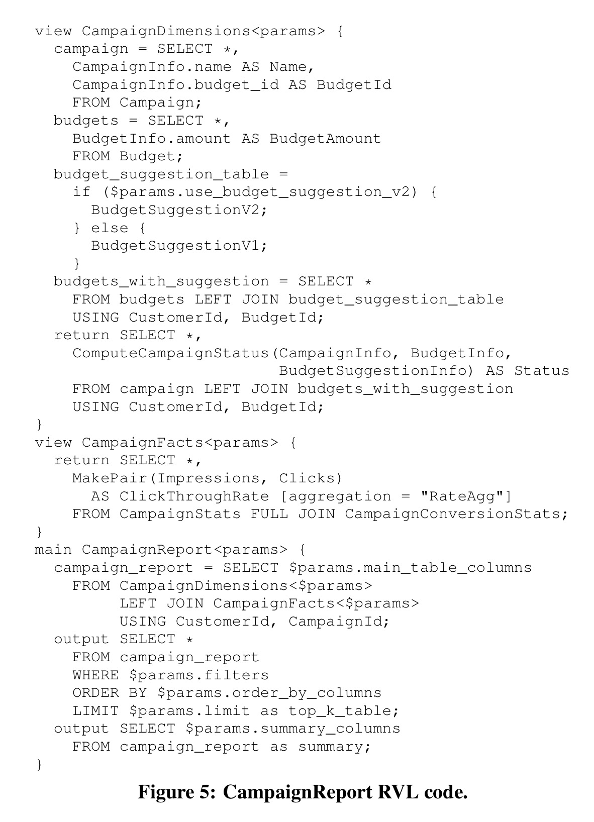
Let’s put it all together with a more realistic worked example. Here we see a set of tables from the campaign management domain. CampaignStats and CampaignConversionStats are actually Mesa fact tables.
The following RVL code defines a CampaignReport main (invocable) view over the tables:
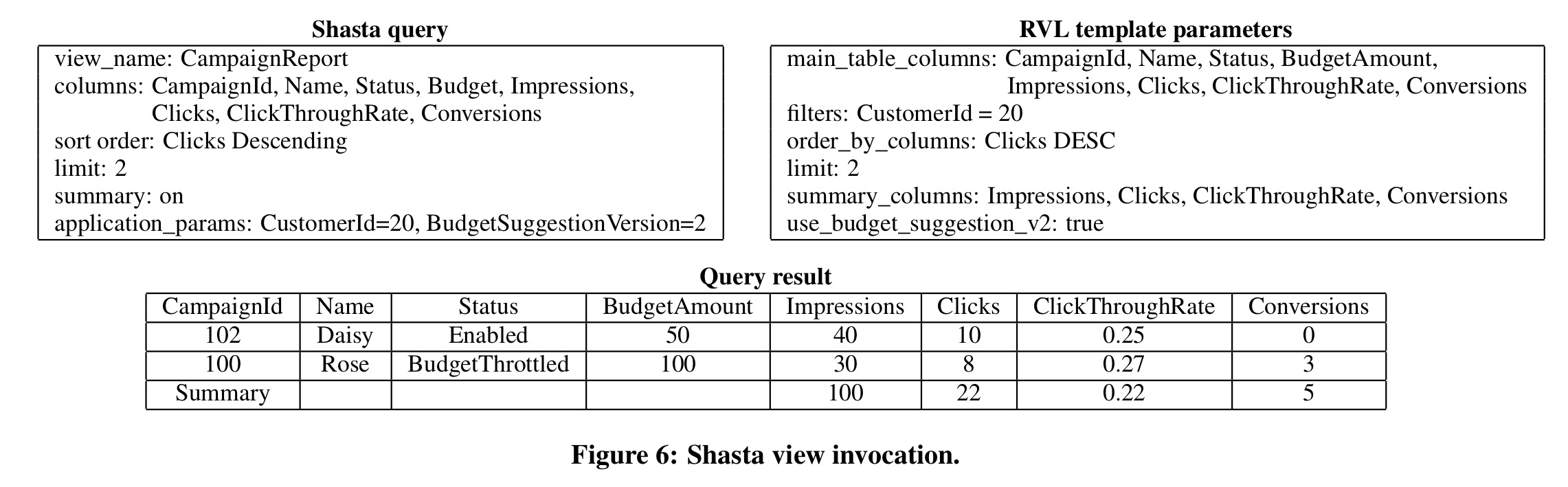
Given the view template, a typical Shasta query and results might look like this:
The last word
Shasta solves two significant challenges:
- Enabling complex data transformations to be expressed in a way that scales to large engineering organisations and supports dynamic generation of online queries with rich query-time parameters.
- Executing the resulting complex queries – which might e.g. read from diverse data stores and join 50 or more tables – reliably at low latency.
Using RVL, user queries can be stated succinctly and view definitions can naturally capture the dynamic nature of applications. At the system level, Shasta leverages a caching architecture that mitigates the impedance mismatch between stringent latency requirements for reads on the one hand, and the underlying data store being mostly write-optimized on the other.