Time-adaptive sketches (Ada Sketches) for Summarizing Data Streams Shrivastava et al. SIGMOD 2016

More algorithm fun today, and again in the context of data streams. It’s the 3 V’s of big data, but not as you know it: Volume, Velocity, and Var… Volatility. Volatility here refers to changing patterns in the data over time, and that can make life awkward if you’re trying to extract information from a stream. In particular, the authors study the heavy hitters problem, but with a twist: we want to give more weight to recent trends.

In most applications that involve temporal data, most recent trends tend to be most informative for predictive purposes…. For instance, most recent variations in credit history are much stronger indicators of a person’s ability to make loan payments compared to variations in credit history from the distant past.

Time-adaptive sketches generalize sketching algorithms and have the property that they retain counts of heavy hitters with good accuracy, while also providing provable time-adaptive guarantees. Coming in at 16 pages, the essence of the paper, especially if you’re familiar with count-min sketches is this: instead of increasing counters by 1 every time you see an item, increase them by f(t), where f(t) is a monotone function in time. When you want to extract count estimates for time t, divide by f(t). The authors experiment with a linear function f(t) = at, for fixed a (0.5), and also an exponential function f(t) = a^t for fixed a (1.0015). Both gave good results.

Finishing the write-up here though would be to short-change you. We’re interested in why this works, and what guarantees it gives. Plus the paper also gives an excellent tour through some of the prior approaches to solving the heavy hitters problem. Let’s start there, with a very quick recap on the basic Count-Min Sketch (CMS) algorithm.

Count-Min Sketch

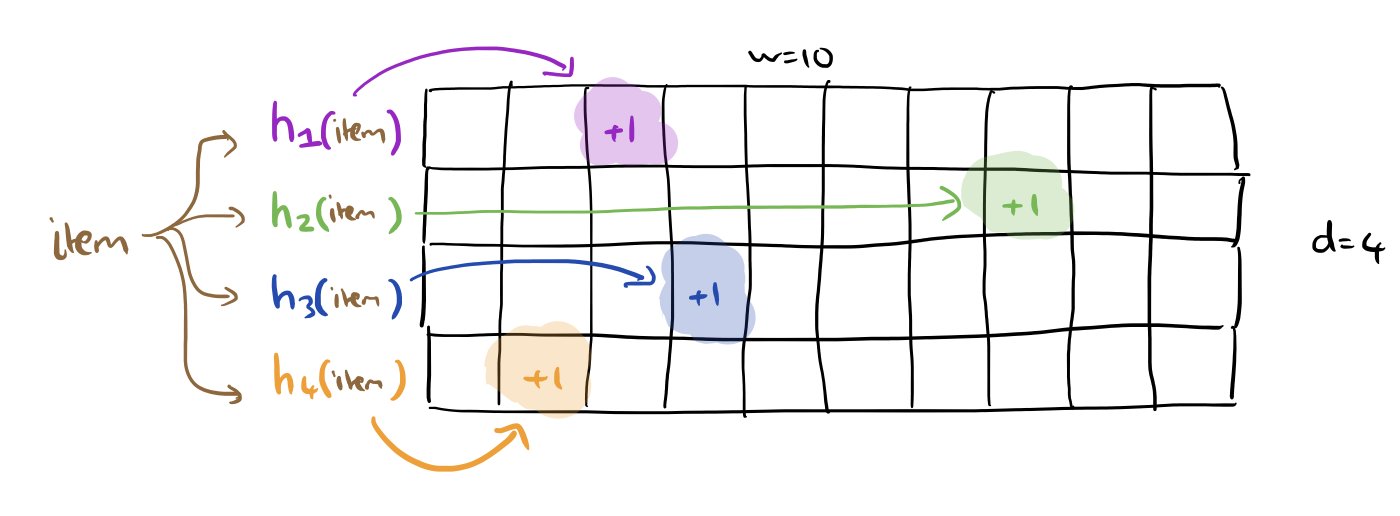
Create an integer array initialised to zeros that is w wide and d deep. Take d pairwise independent hash functions, h₁,…,h_d and associate one with each row of the table, these functions should produce a value in the range 1..w. When a new value is seen, for each row of the table, hash the value with the corresponding hash function, and increment the counter in the indicated array slot.

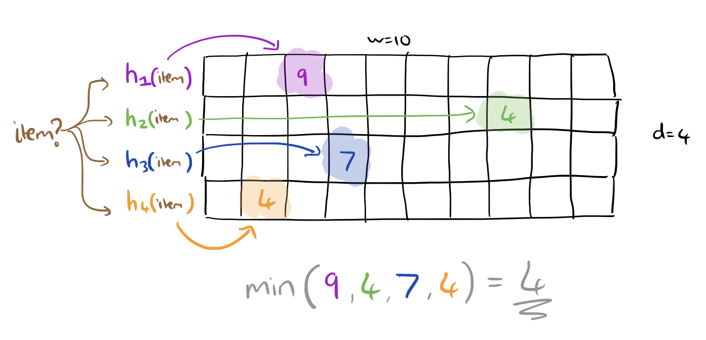
If you want to know the estimate of how many instances of a given value have been seen, hash the value as previously and look up the counter values that gives you in each row. Take the smallest of these as your estimate.

Hokusai – nearly but not quite

Hokusai-sketching (Matusevych et al. 2012) introduced an item aggregation algorithm for constructing time-adaptive sketches.

Hokusai uses a set of Count-Min sketches for different time intervals, to estimate the counts of any item for a given time or interval. To adapt the error rate temporally in limited space, the algorithm uses larger sketches for recent intervals and sketches of smaller size for older intervals.

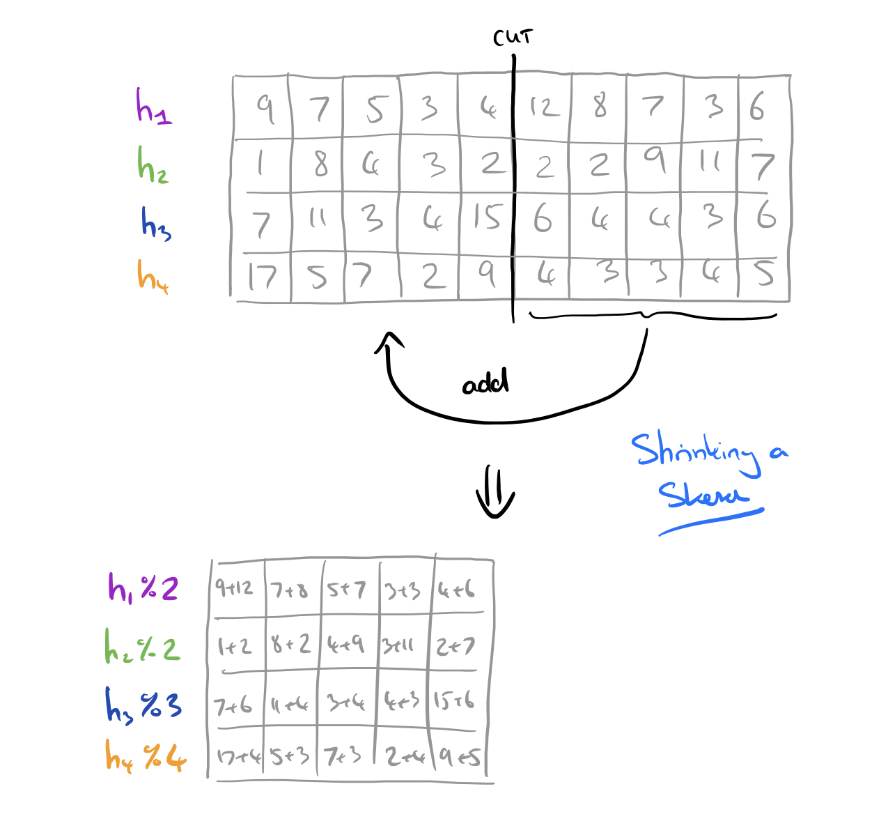
At the end of a time interval (e.g T), a sketch needs to be moved into the next-sized-down sketch, (the one for T–1). Hokusai has a very elegant way of doing this: at each rung on the ladder, sketch widths are halved. You can therefore compress a larger sketch into a smaller one by simply adding one half of the sketch to the other, and also halving the hash function ranges using modulo 2 operations.

Although this idea of having different-size sketches for different time intervals is reasonable and yields accuracies that are time-adaptive, it comes with several inherent shortingcomings.

Inspiration – Dolby noise reduction!

This might date some of The Morning Paper readers – do you remember Dolby B noise reduction? And then the exciting introduction of Dolby C? Some of us grew up with music on cassette tapes, and Dolby Noise Reduction was ever present.

When recording, Dolby systems employ pre-emphasis – artificially boosting certain parts of the input signal. On playback, the reverse de-emphasis translation restores the original signal levels. This process helps to improve the signal-to-noise ratio and combat tape hiss.

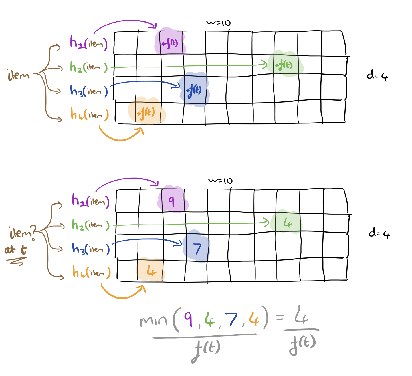
We exploit the fact that Count-Min Sketch (CMS)… has better accuracy for heavy-hitters as compared to the rest of the items. While updating the sketch we apply pre-emphasis and artificially inflate the counts of more recent items compared to older ones, i.e., we make them heavier with respect to the older items. This is done by multiplying updates c_i^t with f(t), which is any monotonically increasing function of time t. Thus, instead of updating the sketch with c_i^t we update the sketch with _f(t) x c_i^t. The tendency of the sketch is to preserve large values. This inflation thus preserves the accuracy of recent items, after artificial inflation, compared to the older ones.

On querying of course, the de-emphasis process must be applied, which means dividing the results by f(t) to obtain the estimate of item i at time t. In the absence of collisions, as with the base CMS, counts are estimated exactly. Consider a CMS with only one row, and the case when two independent items i and j collide. We see c_i^t instances of i, and c_j^t’ instances of j. With plain CMS, we would over-estimate the count for i by c_j^t’, whereas with the pre-emphasis process we overestimate by (f(t) x c_j^t)/f(t’)). Therefore it is easy to see that more recent items suffer less compared to older items.

Adaptive CMS

The Adaptive Count-Min Sketch algorithm (Ada-CMS), is just CMS but with the update and query mechanisms adapted to use the pre-emphasis and de-emphasis mechanism just described. Note that when f(t) = 1 we obtain the original CMS algorithm.

By choosing appropriate f(t) functions, we can tailor the behaviour for different situations.

One major question we are interested in is "Given a fixed space and current state of time T, what are the values of time t ≤ T where Ada-CMS is more accurate than vanilla CMS?

For a given w and d, we can see as a start that the expected error of Ada-CMS will be less than CMS if:

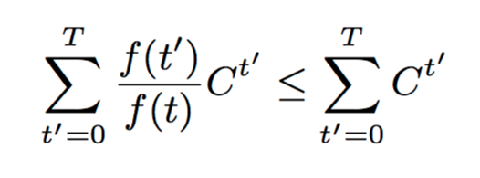
For t=T this will always be true (due to the monotonicity requirement on f(t)). The upper bound on the error with vanilla CMS is &sqrt;T, so Ada-CMS wins when its error is less than this.

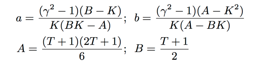
To illustrate a reasonable scenario, suppose we want the errors with Ada-CMS to be never off by a factor γ away from that of vanilla CMS ∀ t. This ensures that we guarantee accuracy within a factor γ of what the original CMS would achieve to even very old heavy hitters. In addition, we want to be more accurate than CMS on all recent time t > K, for some desirable choice of K.

With a couple of simple manoeuvres (see section 5.2), this turns into solving the following pair of simultaneous equations:

Other applications

The pre-emphasis and de-emphasis technique can be used in a number of other scenarios. The authors show an example with the Lossy Counting algorithm, and also how it can be applied to range queries (see §6).

Evaluation

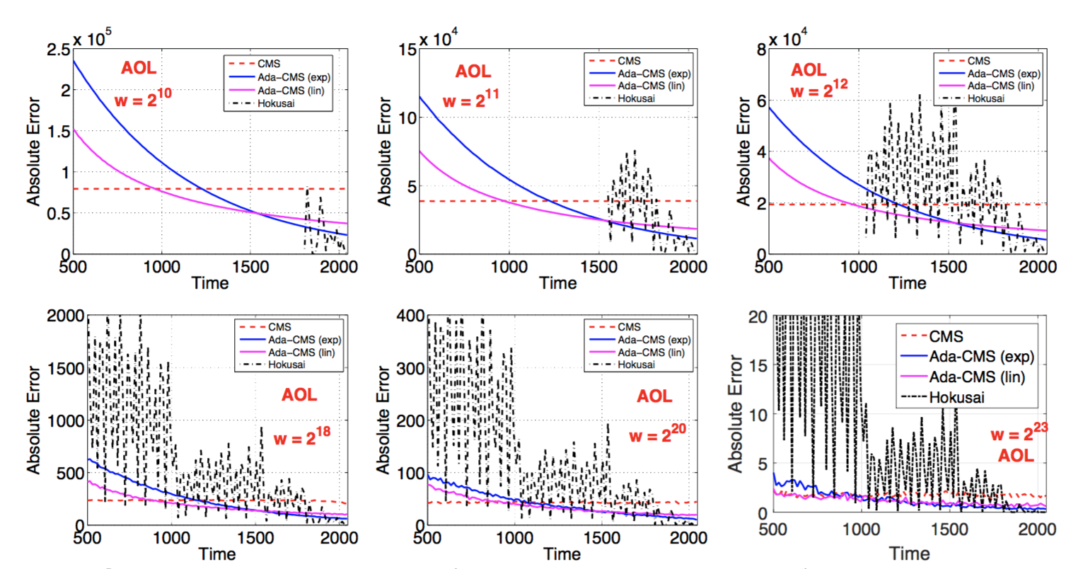
Experimental evaluation is undertaken with two real-world streaming datasets from AOL (36M search queries with 3.8M unique terms) and Criteo (150K unique categorical terms). Comparison is undertaken between vanilla CMS, the Hokusai algorithm, Ada-CMS with a linear function (f(t) = 0.5t), and Ada-CMS with an exponential function (f(t)=1.0015^t). In all cases d = 4, and w was varied from 2¹⁰ to 223 to see the impact of varying range sizes. Here are the results for the AOL dataset:

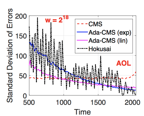
Here’s the standard deviation of those errors with w=2¹⁸:

The Last Word

The proposed integration of sketches with pre-emphasis and de-emphasis, as we demonstrate, posseses strong theoretical guarantees on errors over time. Experiments on real datasets support our theoretical findings and show significantly superior accuracy and runtime overhead compared to the recently proposed Hokusai algorithm. We hope that our proposal will be adopted in practice, and it will lead to further exploration of the pre-emphasis and de-emphasis idea for solving massive data stream problems.