Dynamic Time Warping averaging of time series allows faster and more accurate classification – Petitjean et al. ICDM 2014
For most time series classification problems, using the Nearest Neighbour algorithm (find the nearest neighbour within the training set to the query) is the technique of choice. Moreover, when determining the distance to neighbours, we want to use Dynamic Time Warping (DTW) as the distance measure.
Despite the optimisations we looked at earlier this week to improve the efficiency of DTW, the authors argue there remain situations where DTW (or even Euclidean distance) has severe tractability issues, particularly on resource constrained devices such as wearable computers and embedded medical devices. There is a great example of this in the evaluation section, where recent work has shown that it is possible to classify flying insects with high accuracy by converting the audio of their flight (buzzing bees, and so on).
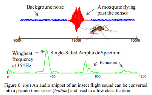
The ability to automatically classify insects has potential implications for agricultural and human health, as many plant/human diseases are vectored by insects. The promising results presented in [31] are demonstrated in the laboratory settings, and exploit large training datasets to archive high accuracy. However, field deployments must necessarily be on inexpensive resource-constrained hardware, which may not have the ability to allow nearest-neighbor search on large training datasets, up to hundreds of times a second. Thus we see this situation as an ideal application for our work.
The question thus becomes: given that we know we want to use NN-DTW classification, how do we reduce the resources required? Since we’re using nearest neighbour, the cost of classification is a function of the number of neighbours that we have to compute the distance to. In the terminology used in the time series world, this is referred to as the size of the training set. The ‘training‘ set is what we actually use to classify query sequences. I find this terminology confusing compared to machine learning where the training set is used to train a model, but the training set is not used for actual classification (only the trained model).
How can we reduce the size of the training set? Using data editing techniques you can create a smart data set with an error rate as low as a much larger random subset. (See yesterday’s paper for example). For the resource constrained devices considered in this work, even this only partly mitigates the problem.
What if we clustered the neighbours belonging to each class and then compared the query to the centroids of the clusters? This is the Nearest Centroid Classifier (NCC) approach, in which the training set size is reduced down to one ‘average’ example per class.
The Nearest Centroid Classifier (NCC) is an apparent solution to this problem. It allows us to avail of all of the strengths of the NN algorithm, while bypassing the latter’s substantial space and time requirements.
As well as being faster, in some circumstances the nearest centroid classifier is also more accurate than a nearest neighbour classifier! A double win.
The idea that the mean of a set of objects may be more representative than any individual object from that set dates back at least a century to a famous observation of Francis Galton. Galton noted that the crowd at a county fair accurately guessed the weight of an ox when their individual guesses were averaged. Galton realized that the average was closer to the ox’s true weight than the estimates of most crowd members, and also much closer than any of the separate estimates made by cattle experts.
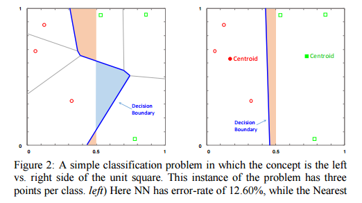
Consider a unit square with data points uniformly distributed within it, and in which the goal is to classify whether a point falls on the left-hand side or the right-hand side of the square. In this case, across a variety of data set sizes the nearest centroid algorithm beats the nearest neighbour algorithm – the effect is small, but it is statistically significant.
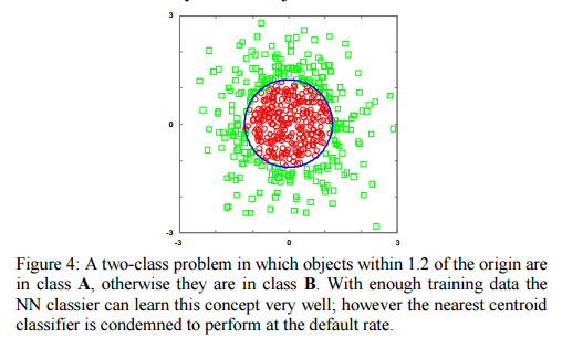
This doesn’t work in all cases – for example in the ‘Japanese flag’ dataset NN gets better with more data points, whereas NCC never improves beyond the default rate.
In spite of the existence of such pathological cases, the Nearest centroid classifier often outperforms the NN algorithm on real datasets, especially if one is willing (as we are) to generalize it slightly; for example, by using clustering to allow a small sample of centroids [within each class], rather than just one. Thus our claim is simply:
- Sometimes NCC and NN can have approximately the same accuracy, in such cases we prefer NCC because it is faster and requires less memory.
- Sometimes NCC can be more accurate than NN, in such cases we prefer NCC because of the accuracy gains, and the reduced computational requirements come “for free”
Take the ‘Japanese flag’ dataset example – it’s easy to see that a single centroid is optimal for the circle/red class, but to identify the outer/green class we need to arrange examples (for example, eight in an octagon around the circle) to carve out a decision boundary that approximates the true circular decision boundary. A similar thing happens in the insect surveillance example given earlier. Suppose you want to classify mosquitoes. Creating a single template that attempts to represent both males and females ends up representing neither. But by using two templates, one for each sex, we do much better.
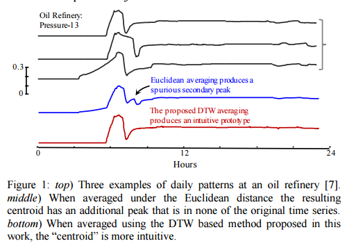
Problem solved !? Not quite… there’s just one small snag left: the concept of a centroid isn’t defined for time series. “Even if we consider only objects that have a very low mutual DTW distance, if we attempt to average them the result will typically be ‘neither fish nor fowl,’ resembling none of the parent objects.” Fortunately, the authors show how to compute a useful “centroid” in this paper.
Finding a meaningful average for time series
Computational biologists have long known that averaging under time warping is a very complex problem, because it directly maps onto a mutiple sequence alignment: the “Holy Grail” of computational biology… Finding the solution to the multiple alignment problem (and thus finding the average of a sequence) has been shown to be NP-complete with the exact solution requiring O(LN) operations for N sequences of length L.
How bad is O(LN)? 45 sequences of length 100 would require more operations than the number of particles in the universe!
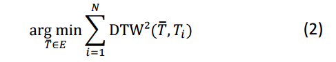
We can cast it as an optimisation problem: given a set of time series D = {T1,…TN} in a space E induced by Dynamic Time Warping, the average time series Tavg is the time series that minimizes:
Many attempts at finding an averaging method for DTW have been made since the 1990s…
The approach that outperforms all others on the datasets of the UCR Archive is DTW Barycenter Averaging (DBA). “In particular, it always obtained lower residuals than the state-of-the-art methods, with a typical margin of about 30%, making it the best method to date for time series averaging for DTW.”
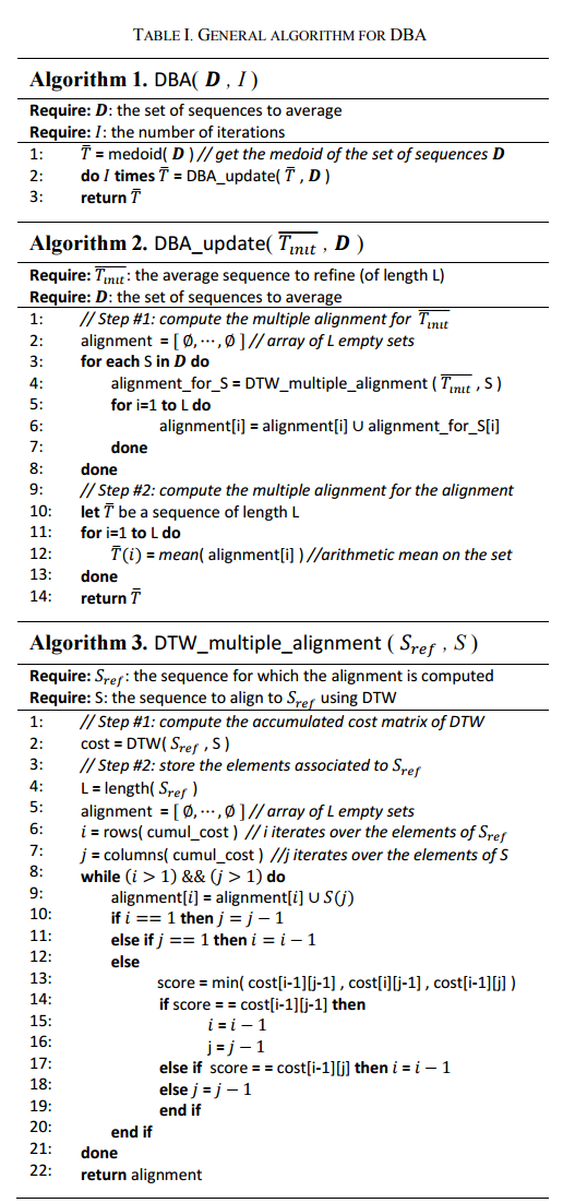
DBA is an iterative algorithm that refines an average sequence Tavg on each iteration following an expectation maximization scheme. Each iteration has two phases:
- For every sequence S in the dataset D to be averaged, find the best multiple alignment under DTW of S with Tavg.
- Update Tavg as the best average sequence consistent with M.
At the start of the algorithm, Tavg is seeded with the medoid member of D – the member in D that has the minimum sum-of-squares distance from all other members of the set. The authors prove (in an appendix) that this algorithm always converges. It is perhaps easiest to understand the algorithm from its pseudocode:
Classification results
Returning to the insect classification example, the authors recorded about 10,000 flights and created a dataset by randomly choosing 200 examples of each class (male/female). The dataset was then split into two balanced train/test datasets of the same size.
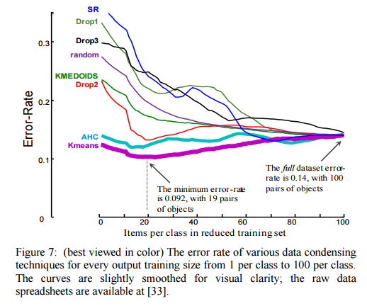
As we can see in figure 7, our algorithm is able to achieve a lower error-rate using just two items per class, than by using the entire training dataset. This is an astonishing result. The curves for the other approaches are more typical for data condensing techniques, where we expect to pay a cost (in accuracy) for the gains in speed. The error rate for our approach is minimized at 19 items per class, suggesting we can benefit from some diversity in the training data.
To see if the results generalised, the method was then tested against all of the datasets in the UCR time series archive.
TABLE IV shows the average rank of all algorithms over the datasets of [the UCL time series archive]… These results show unanimously that the methods that use an average sequence (K-means and AHC) significantly outperform the prior
state of the art.
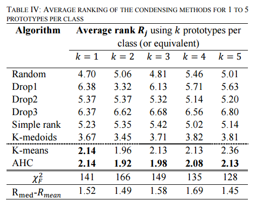
(K-means is the combination of DBA with K-means clustering, and AHC is the combination of DBA with agglomerative hierarchical clustering (AHC), which progressively merges the most similar clusters until all the objects are part of the same cluster).
On average across these datasets the k-means clustering approach needs a training set only 29% of the size of the full dataset to achieve equal or better performance than a nearest neighbour classifier using the full dataset.