Ernest: Efficient Performance Prediction for Large-Scale Advanced Analytics – Venkataraman et al. 2016

With cloud computing environments such as Amazon EC2, users typically have a large number of choices in terms of the instance types and number of instances they can run their jobs on. Not surprisingly, the amount of memory per core, storage media, and the number of instances are crucial chocies that determine the running time and thus indirectly the cost of running a given job.

Ernest takes on the challenge of predicting the most efficient configuration for large advanced analytics applications in a heterogeneous multi-tenant environments. It might be that you have a certain budget, and want to minimize the running time given that budget, or perhaps you have a time limit, and want to complete the job as cheaply as possible within that time limit. Either way, exhaustively trying all of the combinations to find out which work the best isn’t really feasible.

Ernest observes a small number of training runs on subsets of the data, and then builds a performance model that predicts how well the job will perform in different configurations.

Our evaluation shows that our average prediction error is under 20%, and that this is sufficient for choosing the appropriate number or type of instances. Our training overhead for long-running jobs is less than 5% and we also find that using experiment design improves prediction error for some algorithms by 30-50% over a cost-based scheme. Finally, using our predictions we show that for a long-running speech recognition pipeline, finding the appropriate number of instances can reduce cost by around 4x compared to a greedy allocation scheme.

I was especially excited to read about this work since one of the companies I work with, Skipjaq, is also using machine learning to optimise applications (throughput, latency, cost) and has been seeing really impressive uplifts on real customer applications leading to significant cost savings. Skipjaq doesn’t yet optimize the same kind of advanced analytics applications that Ernest is targeting, but the results on even very traditional looking applications have proven to me just how powerful these kinds of approaches can be.

Let’s take a look at how Ernest works its magic…

Building a Performance Model

At a high level performance modeling and prediction proceeds as follows: select an output or response variable that needs to be predicted and the features to be used for prediction. Next, choose a relationship or model that can provide a prediction for the output variable given the input features… We focus on machine learning based techniques in this paper.

The main steps in building a predictive model are determining the data points to collect; determining what features should be derived from the training data; and performing feature selection to pick the simplest model that best fits the data.

Advanced analytics workloads are numerically intensive and hense are sensitive to the number of cores and bandwidth available, they are also expensive to run on large datasets.

…we observe that developers have focused on algorithms that are scalable across machines and are of low complexity (e.g. linear or quasi-linear). Otherwise, using these algorithms to process hug amounts of data might be infeasible. The natural outcome of these efforts is that these workloads admit relatively simple performance models.

The authors note that only a few communication patterns repeatedly appear in analytics jobs.

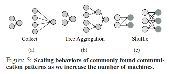
(a) the all-to-one or collect pattern in which data from all partitions is sent to one machine
(b) the tree aggregration pattern where data is aggregated using a tree-like structure
(c) the shuffle pattern where data goes from many source machines to many destinations

The model is built using terms related to these computation and communication patterns. It has four components:

• θ₀ – a fixed cost term representing the amount of time spent in serial computation
• θ₁ x (scale/machines) – to capture the parallel computation time for algorithms whose computation scales linearly with the data
• θ₂ x log(machines) – to model communication patterns like aggregation trees
• θ₃ x machines to capture the all-to-one communication pattern and fixed overheads like scheduling / serializing tasks.

time = θ₀ + θ₁.scale/machines + θ₂.log(machines) + θ₃.machines

Note that as we use a linear combination of non-linear features, we can model non-linear behavior as well.

The goal is to find the values of θ₀..θ₃ that best fit the training data.

(Aside: I’d love to see a comparison that shows how well this model performs against the Universal Scalability Law which has two coefficients α and β : C(N) = N / ( 1 + α(N-1) + βN(N-1) ) ).

Given these features, we then use a non-negative least squares (NNLS) solver to find the model that best fits the training data. NNLS fits our use case very well as it ensures that each term contributes some non-negative amount to the overall time taken… NNLS is also useful for feature selection as it sets coefficients which are not relevant to a particular job to zero.

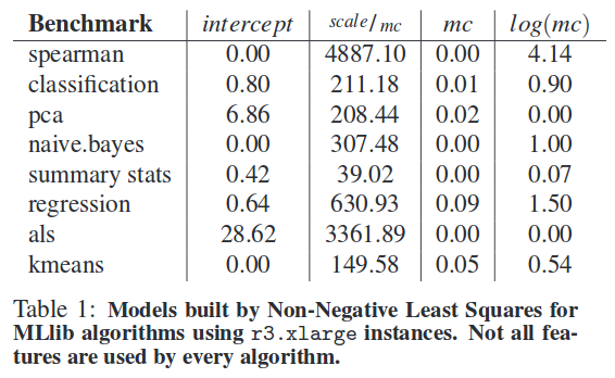
The authors trained an NNLS model using just 7 data points on all of the machine learning algorithms from MLlib in Apache Spark 1.2. The final model parameters are show below – notice that not all features are used by every algorithm, and the contribution of each term differs with every algorithm.

Some complex algorithms may not fit this model. Ernest uses cross-validation to figure out when a model is not fitting well. “There are a number of methods to do cross-validation, and as our traning data size is small, we use a leave one out cross validation scheme.” Given m training data points, m cross-validation runs are performed where each run uses m-1 points as training data and tests the model on the left-out data point.

An example where the default model does not predict behaviour well is the GLM classification implementation in Spark MLlib. Here the aggregation uses two stages, and √n tasks for n partitions of data in the first stage.

Extending the model in Ernest with additional terms is simple and in this case we can see that adding the √n term makes the model fit much better.

Finding Parameters with Optimal Experiment Design

To improve the time taken for training without sacrificing the prediction accuracy, we outline a scheme based on optimal experiment design, a statistical technique that can be used to minimize the number of experiment runs required.

The basic idea is to determine the data points that give us the most information to build an accurate model. Suppose the space we want to explore is from 1 to 5 machines, and from 1% to 10% of the data (in steps of 1%). That gives us 5×10 = 50 different possible feature vectors.

If we have m training points, each with an n-dimensional feature vector a, then the overall variance of the estimator is given by

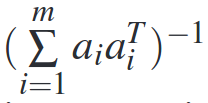
Important to note is that this depends only on the feature vectors used for the experiment, and not on the actual measured values for the model being estimated.

In optimal experiment design we choose feature vectors (i.e. _a_i) that minimize the estimation error. Thus we can frame this as an optimization problem where we minimize the estimation error subject to constraints on the number of experiments. More formally, we can set λ_i as the fraction of times an experiment is chosen and minimize the trace of the inverse of the covariance matrix:

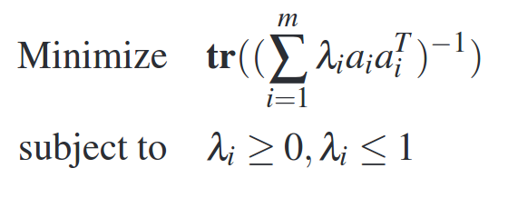
The features vectors (e.g. scale, machines) can be fed into this experiment design setup and then only those experiments whose λ values are non-zero are run.

To account for the cost of an experiment we can augment the optimization problem we setup above with an additional constraint that the total cost should be less than some budget. That is, if we have a cost function which gives us a cost c_i for an experiment with scale s_i and m_i machines, we add a constraint to our solver that

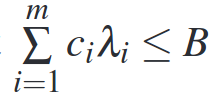
where B is the total budget.

Implementation and Evaluation

Ernest is implemented in Python with a job submission tools, a training data selection process which implements experiment design using a CVX solver, and a model builder that using NNLS from SciPy. “Even for a large range of scale and machine values we find that building a model takes only a few seconds and does not add any overhead.”

To deal with the problem of stragglers, Ernest launches a small percentage of extra instances and discards the worst performing among them before running the user’s job. “In our experiments with Amazon EC2 we find that even having a few extra instances can be more than sufficient in eliminating the slowest machines.”

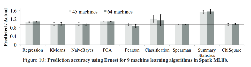
The main results from the evaluation are as follows:

• Ernest predicts run times with less than 20% error on most workloads, with less than 5% overhead for long running jobs (training time is below 5% of the actual running time of the job).

• Using the predictions from Ernest, a 4x cost-reduction is possible for the speech pipeline by choosing the optimal number of instances
• For a given training budget, experiment design improves accuracy by 30-50% for some workloads when compared to a cost-based approach
• By extending the default model, Ernest is also able to accurately predict running times for sparse and randomized linear algebra operations.