Functional Reactive Animation – Elliott & Hudak 1997
This is the paper widely acknowledged to have given birth to (Functional) Reactive Programming or FRP. The challenge that Elliott and Hudak faced was to provide an elegant and expressive way to specify animations without resorting to tedious frame-by-frame constructions. A key insight is that animations are all about how something changes over time, and time is conceptually continuous. Fran makes the notion of continuous behaviours first class in the programming model.
The construction of richly interactive multimedia animations (involving audio, pictures, video, 2D and 3D graphics) has long been a complex and tedious job. Much of the difficulty, we believe, stems from the lack of sufficiently high-level abstractions, and in particular from the failure to clearly distinguish between modeling and presentation, or in other words, between what an animation is and how it should be presented… The benefits of a modeling approach to animation are similarto those in favor of a functional (or other declarative) programming paradigm, and include clarity, ease of construction, composability, and clean semantics.
The modeling approach also makes animations easier to author, and easier to optimize. Fran is a collection of recursive data types, functions, and primitive graphics routines brought together around four central concepts: behaviors, events, declarative reactivity, and polymorphic media. The most novel aspect of Fran is its implicit treatment of time.
Behaviours (temporal modeling)
A behaviour is a value that can vary over time.
Behaviors are first-class values, and are built up compositionally; concurrency (parallel composition) is expressed naturally and implicitly.
The simplest primitive behaviour is time itself. And cos time, for example, is a behaviour that varies as the cosine of time, created by lifting the cosine function to apply to behaviours. We can create a simple animation that changes the shape of a square over time as follows:
bigger (cos time) square
bigger scales its second argument by the amount specified in the first argument. Since the first argument is a behaviour, the result is also a behaviour. Using the over function as an infix operator we can place a circle on top whose size changes as the sine of time:
bigger (sin time) circle `over` bigger (cos time) square
Event Modeling
Events are also first class values in Fran. They can represent actual events in the external world (for example, a button press), and they can also be expressed as predicates (for example, based on proximity). Events are ‘what’, ‘when’ pairs. The when component is a lower bound on the time of the event – for examplelbp t0 represents the first left button press (‘what’), occurring after time t0.
Declarative reactivity
Here we see the first use of the ‘reactive’ term…
Many behaviors are naturally expressed in terms of reactions to events. But even these “reactive behaviors” have declarative semantics in terms of temporal composition, rather than an imperative semantics in terms of the state changes often employed in event-based formalisms.
b `untilB` e
Exhibits behaviour b until event e occurs, after which it behaves according to the behaviour associated with e. Using this we can describe a colour cycle as follows:
    colorCycle t0 =
      red `untilB` lbp t0 *=> \t1 ->
      green `untilB` lbp t1 *=> \t2 ->
      colorCycle t2
update: fixed > vs > in the above, thanks David for pointing out the issue.
Fran is implemented in Haskell, where \x -> … defines a lambda function with bound variable x. This reactive behaviour can thus be interpreted as:
- show red until the first left-button press after time t0, and then
- show green until the first left-button press after time t1 (the time of the previous lbp), and then
- repeat the color cycle starting at time t2 (the time of the second lbp)
Polymorphic Media
The variety of time-varying media (images, video, sound, 3D geometry) and parameters of those types (spatial transformations, colors, points, vectors, numbers) have their own type-specific operations (e.g. image rotation, sound mixing, and numerical addition), but fit into a common framework of behaviors and reactivity. For instance, the “untilB” operation used above is polymorphic, applying to all types of time-varying values.
Examples
The paper includes a formal semantics of behaviours and events, as well as some implementation notes that describe an ‘interval analysis’ technique for detecting predicate events. We’ll look in more detail at design and implementation considerations for reactive frameworks later this week. For now, let’s just look at a few more code examples to get a feel for the expressivity of modeling that behaviours and events support.
A behaviour that varies smoothly and cyclically between -1 and 1:
wiggle = sin (pi * time)
And a behaviour that builds on this to smoothly vary between a high and low value:
wiggleRange lo hi =
  lo + (hi - lo) * (wiggle + 1)/2
A red pulsating ball:
pBall = withColor red
          (bigger (wiggleRange 0.5 1) circle)
Behaviours are composable, as we’ve been seeing already. Let’s use pBall as a building block…
rBall = move (vectorPolar 2.0 time)
             (bigger 0.1 pBall)
“which yields a ball moving in a circular motion with radius 2.0 at a rate proportional to time. The ball itself is the same as pBall (red and pulsating), but 1/10 the original size.”
An image that tracks the position of the mouse:
followMouse im t0 = move (mouse t0) im
As a final example, let’s develop a modular program to describe “bouncing balls.” First note that the physical equations describing the position y and velocity v at time t of an object being accelerated by gravity g are:
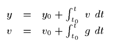
where y0 and v0 are the initial position and velocity, respectively of the object at time t0. In Fran these equations are simply:
y = lift0 y0 + integral v t0
x = lift0 v0 + integral g t0
update: corrected typo in the x expression, thanks to zteve for pointing it out.
Next we define a function bounce that, in addition to computing the position of an object based on the above equations, also determines when the ball has hit either the floor or the ceiling, and if so reverses the direction of the ball while reducing its velocity by a certain reciprocity, to account for loss of energy during the collision…
(See figure 1 in the paper for the bounce code). Using bounce we can also simulate horizontal movement if we simply use 0 for acceleration. Here’s a bouncing ball in a box:
moveXY x y
  (withColor green circle)
where
  x = bounce xMin xMax x0 vx0 0 t0
  y = bounce yMin yMax y0 vy0 g t0
See the full paper for further examples.