Efficient Algorithms for Public-Private Social Networks – Chierichetti et al. 2015
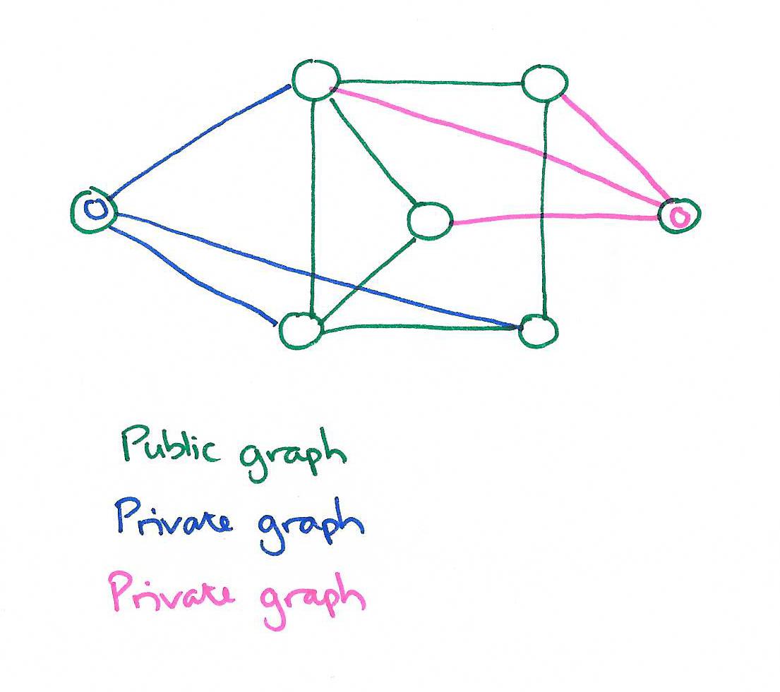
Today’s choice won a best paper award at KDD’15. The authors examine a number of algorithms for computing graph (network) measures in the context of social networks that enable private groups and connections. These are characterised by a large public graph G=(V,E), and for each user (node) u ∈ V, a private graph Gu. All the nodes in Gu are themselves members of the public graph (no private users/nodes). Furthermore, each node in the private graph of u is at most distance 2 from u. This is “sufficient to capture many interesting privacy settings.”
Consider the case of sharing a private circle in Google+. When a node u builds a private circle, it can choose that the members of the circle are visible to the rest of the circle. Consider two members v and w of this circle that are not in each others’ public or private circles. Then the edge (u, v) is private to w and the edge (u,w) is private to node v. In other words, (u,w) ∈ Gv and (u, v) ∈ Gw, but neither of v nor w is connected to the other in the public graph, or in either or their private graphs.
A study of 1.4M New York City Facebook users found that 52.6% of them hid their friends list.
To illustrate the scenario further, consider a social recommendation algorithm. The social network provider could use only the public portion of the network to run the algorithm and build recommendations; this will easily ensure privacy for all the users. But, this will not benefit nodes whose edges are overwhelmingly private; as noted in the NYC example, there can be several such nodes. Alternatively, social network providers can, naively speaking, run the algorithm once for each user, on the union of the public portion of the network and the user’s private network. This also clearly respects the overall privacy requirements, however, it is grossly inefficient.
An algorithm in the public-private model is said to be efficient if it can compute a function on G ∪ Gu in time proportional to the size of Gu. You are allowed to preprocess G and store the results. The authors discuss efficient public-private algorithms for both sketching (size of the reachability tree, and centrality measures) and sampling (shortest-paths, pair-wise node similarities, and corellation clustering) approaches. When the authors benchmark their algorithms against the naive approach (re-running the algorithm on G ∪ Gu) they unsurprisingly run orders of magnitude more efficiently.
A warm-up problem
The authors demonstrate how to compute the number of connected components as a simple demonstration of the model:
- Preprocess the public graph G to compute its connected components. Assign a component id to each node and store this information along with the total number of connected components.
- To compute the number of connected components in G ∪ Gu, simply count the number of different connected components that Gu connects.
This takes time | Eu | since we only need to scan the edges in Gu.
The follow-on problems are substantially more complex!
Sketching
Some graph sketches are easily composable. If I have a sketch of G and a sketch of H I can simply compose them to give a sketch of G ∪ H. These sketches clearly fit easily in the public-private model.
For other problems such as neighborhood estimation, even though sketches exist and even though they are composable, one has to be careful how to compose them efficiently in the public-private model. This is precisely what we do in this section.
The first example given is computing the size of the reachability tree. For example, using the ‘follow’ relation the size of the reachability tree from a given node gives an indication of the number of people who directly or indirectly follow a given user. The public-private solution to this problem builds on the bottom k sketch.
The basic bottom-k sketch lets you estimate the size of an arbitrary subset of vertices V’ drawn from V. Every node in the full graph is assigned a random number between 0 and 1. The bottom-k sketch of a subset contains the k items with the smallest ranks (assigned random numbers) in the subset. Given this sketch, we can retreive an estimate of the size of the subset as:
- The number of elements in the sketch, if there are less than k (which must be the correct answer, as this is the only way we would fail to have at least k elements)
- (k-1)/bk otherwise, where bk is the largest value (assigned random number) in the sketch
We can use these sketches to estimate the size of the reachability tree for a given node:
- Start out by assigning each node a random number between 0 and 1, and associate with each node a bottom-k sketch of its immediate neighbours (nodes it is connected to via an outbound edge). For node v, we denote this initial sketch S(v,0).
- Perform D iterations of the following process, where D is the diameter of the graph: for each node v, construct the union of v’s bottom-k sketch and the bottom-k sketches of all v’s out-neighbours. Let v’s new sketch S(v,i) be the bottom-k members (i.e., the kth smallest members) of this union.
At the end of this process, S(v,D) is a sketch of all nodes in the reachability tree of v (and thus we can estimate its size). This represents our pre-processing of the public graph G. Given these sketches, the goal now is to compute the size of the reachability tree for the public-private graph G ∪ G/u. This can be done solely by recomputing the sketches for u and its immediate out-neighbours.
One of the rules for constructing a public-private graph is that each node in the private graph of u is at most 2 distant from u. That constraint comes in handy… Starting with u, consider the set of nodes that are its out-neighbours. The set of nodes that are the out-neighbours of those out-neighbours are distance 2 away, and so we already have correct sketches for their reachability trees. Thus we can create new sketches for the out-neighbours v of u by combining these distance-2 sketches with a sketch of the new neighbours of v introduced by Gu.
…when we add a few outgoing edges to a node we just need to add the reachability tree of the new neighbors and the new neighbors to obtain the new reachability tree.
With these updated neighbour sketches, we can apply the same logic to get an updated sketch for u itself. Because we are able to ignore in-neighbours when computing reachability, this is sufficient.
I’ve tried here to give an intuitive understanding of the algorithm (you can be the judge as to whether I’ve succeeded!). For a more formal and complete treatment see the details in the paper.
Three centrality meaures are also considered: closeness centrality, Lin’s centrality, and Harmonic centrality. The public-private solutions once more use iteration over bottom-k sketches in a similar manner to the reachability tree size solution.
Sampling
As a representative sampling algorithm, let’s look at All-pair shortest paths. See the paper for details of computing pairwise node similarities and correlation clustering.
In this section we study how to approximate efficiently the distance between any two nodes in the graph in the public-private model. Note that this problem is particularly interesting in our model because the distances between two nodes can change dramatically even if we add a single edge. In this section we assume that the graph is undirected.
As a baseline, take the all-pairs shortest path approximation of Das Sarmas et al.:
- Given a graph with n vertices, we start by by generating subsets of vertices S0, S1, …, Sr with sizes 1,2,…,2r where r = floor(log n).
- For each node v, and all i, compute the closest node vi ∈ Si to v, and the corresponding distance. (I.e., we’re generating shortest paths over ever increasing subsets of the full graph).
To estimate the distance between two nodes v and w we can look at their respective samples. For each i, we look at all the members k ∈ Si, and compute distance(v,k) + distance(k,w) (looking up the distances in our pre-computed data structure). The shortest path estimate is the minimum computed distance over all i and all k.
Know that we have an algorithm for computing shortest paths over G, how can we exploit this to efficiently compute over G ∪ Gu?
The shortest path between u and v must be the minimum of:
- The shortest path between u and v in G (which we already have),
- 1 + the shortest path from each neighbour w of u, where (w,u) is an edge in Gu
- 2 + the shortest path from each second-degree neighbour z of u, where (z,*) is an edge in Gu
Thus we consider at most O(| Eu |) distances, each of which can be estimated in O(log2 n) time.