A higher order estimate of the optimum checkpoint interval for restart dumps – Daly 2004
TL;DR: if you know how long it takes your system to create a checkpoint/snapshot (δ), and you know the expected mean-time between failures (M), then set the checkpoint interval to be √(2δM) – δ.
OK, I grant that today’s paper title sounds like somewhat of a niche interest! It’s another reference from the Distributed GraphLab paper that sent me here, where the authors use Young’s formula to calculate how often Distributed GraphLab should checkpoint its state:
For instance, using a cluster of 64 machines, a per machine MTBF of 1 year, and a checkpoint time of 2 min leads to optimal checkpoint intervals of 3 hrs. Therefore, for the deployments considered in our experiments, even taking pessimistic assumptions for MTBF, leads to checkpoint intervals that far exceed the runtime of our experiments and in fact also exceed the Hadoop experiment runtimes. This brings into question the emphasis on strong fault tolerance in Hadoop. Better performance can be obtained by balancing fault tolerance costs against that of a job restart.
I looked for an open access version of Young’s paper but couldn’t find one. Young’s work was subsequently extended by Daly in today’s paper choice though.
In this study we will expand upon the work begun by Young and continued by Daly in refining a model for quantifying the optimum restart interval that minimizes the total application run time. Our goal is to derive a result in terms of a simple analytic approximation, easily accessible to the application user, with well-defined error bounds.
The approach taken is to generate a cost function that describes the total wall clock time for an execution of an application, and then to determine a minimum. The cost function has four logical components:
the solve time; the dump time; the rework time; and the restart time.
cost = solve + dump + rework + restart
- Solve time is defined as time spent on actual computational cycles towards a final solution. For a system with no interrupts, the wall clock time Tw(τ) consists entirely of solve time.
- Dump time is the overhead spent writing out the checkpoint files required to restart the application after an interrupt.
- Rework time is the amount of wall clock time lost when an application is killed by an interrupt prior to completing a restart dump. It is the amount of time elapsed since the last restart dump was successfully written.
- Restart time is the time required before an application is able to resume real computational work. It includes both the application initialization and any system overhead associated with restarting a calculation after an interrupt.
Young proposed that the optimum checkpoint interval is given by √(2δM), where δ is the time to write a checkpoint file, and M is the mean time to interrupt (MTTI) of the system. Daly’s paper is heavy on the math which I won’t reproduce here (the interesting parts for me are the results, and the modeling process). From the first order model that Daly develops, he is able to refine Young’s model to give the following first-order approximation to the optimum checkpoint interval:
- τopt = √(2δ(M+R)),
For τ+δ (solve time + checkpoint/dump time) being much less than M. This is the same as Young with the addition of the restart time R, which Young did not consider. The first-order model doesn’t cope as well when M becomes smaller (closer to τ+δ), nor does it take into account the fact that failures might occur during restarts.
Daly builds a new (higher-order) cost function taking these additional factors into account. Let’s skip over several pages of math and simulation and go straight to the bottom line:
We found that even though the first-order model predicts a contribution of the restart time R to the selection of the optimum compute interval between checkpoints τopt, the higher order model demonstrates that in fact R has no contribution….
(so Young was right to ignore it!)
Furthermore, we demonstrated that an excellent approximation to τopt, one that guarantees that the relative error in total problem-solution time never exceeds 0.2% of the exact solution time, is given by the first three terms of the perturbation solution
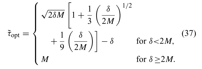
Finally, we observe that the maximum relative error in problem solution time associated with our lowest order perturbation solution, which is equivalent to Young’s model, is less than 5%, even in the worst case when δ = M/2. This is a good rule of thumb for most practical systems, when the value of δ is expected to be small compared to M.
And given all of that the bottom line is as follows:
- If the time it takes to create a dump, δ < M/2 then use τopt = √(2δM) – δ
- Otherwise (it takes longer than M/2 to create a dump), just use τopt = M.
And that’s a handy little rule of thumb to have tucked away in your back pocket…