Dynamics on expanding spaces: modeling the emergence of novelties Loreto et al., ArXiv 2017
Something a little bit left field today to close out the week. I was drawn into this paper by an MIT Technology Review article entitled “Mathematical model reveals the patterns of how innovations arise.” Who wouldn’t want to read about that!? The article (and the expectations set by the introduction to the paper itself) promise a little more than they deliver in my view – but what we do concretely get is a description of a generative process that can produce distributions like those seen in the real world, with new / novel items appearing at the observed rates and following observed distributions. Previous models have all fallen short in one way or another, so the model does indeed seem to teach us something about the process of generating the new.
Novelties are part of our daily lives. We constantly adopt new technologies, conceive new ideas, meet new people, experiment with new situations. Occasionally, we as individuals, in a complicated cognitive and sometimes fortuitous process, come up with something that is not only new to us, but to our entire society so that what is a personal novelty can turn into an innovation at a global level. Innovations occur throughout social, biological and technological systems and, though we perceive them as a very natural ingredient of our human experience, little is known about the processes determining their emergence. Still the statistical occurrence of innovations shows striking regularities that represent a starting point to get a deeper insight in the whole phenomenology.
The plan for today’s post is a little bit different to normal: we’ll start by looking at some of the laws that real world data sets seem to follow under certain conditions, then we’ll jump straight to the part of today’s paper that explains the generative model (skipping the 10+ pages of descriptions of previous models that didn’t quite cut it for one reason or another) before closing out with a brief look at the related (in my mind at least) Social Physics model of Andy Pentland et al. which explains how ideas spread once conceived. The post will therefore be a little bit longer than usual, but I think you’ll find the tour quite interesting!
Benford’s Law
The most counter-intuitive of the laws is Benford’s law, which says that if you look at a real-world distribution of numerical data (for example, population of cities) then you’ll observe the following phenomenon: numbers beginning with 1 are the most common (about 30% of the time), and numbers beginning with 9 are the least common (about 5% of the time). The likelihood of a number beginning with the digit d is 
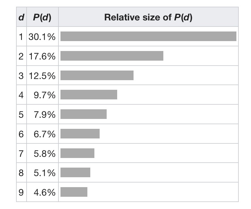
(Source: wikipedia)
The dataset should follow four conditions for the law to hold:
- Values are positive numbers
- Values range over many different orders of magnitude
- Values arise from a complicated combination of largely independent factors
- Values have not been rounded, truncated or otherwise constrained in size
The law has been shown to work in many different scenarios – e.g., city populations, heights of the world’s tallest structures, lengths of rivers, figures in accounts, and so on.
The phenomenon was again noted in 1938 by the physicist Frank Benford, who tested it on data from 20 different domains and was credited for it. His data set included the surface areas of 335 rivers, the sizes of 3259 US populations, 104 physical constants, 1800 molecular weights, 5000 entries from a mathematical handbook, 308 numbers contained in an issue of Reader’s Digest, the street addresses of the first 342 persons listed in American Men of Science and 418 death rates. The total number of observations used in the paper was 20,229. – Wikipedia
It is independent of the units used for the values (e.g., km vs miles) and even of the base (i.e., we don’t have to be using base 10). There’s a good New Scientist article on the law from 1999 entitled ‘The power of one.’
Why it works is complicated. But if the values range over several orders of magnitude, then we could consider that we are drawing random samples from a log scale. Look what happens when you take e.g., values from 1 to 2 inclusive with 0.1 increments and treat them as base 10 logs:
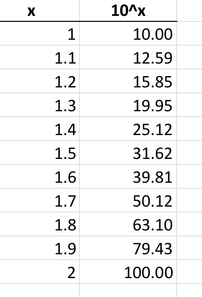
Note that we get numbers that start with the digit ‘1’ all the way up to 1.3 – i.e., about 30% of the time.
Zipf’s Law
Zipf’s law essentially tells us that things which grow large are comparatively rare. In text corpora, it’s the famous result that the frequency of any word is inversely proportional to its rank in the frequency table (so e.g., the 2nd most frequent word appears 1/2 as often as the most frequent, and so on). In the more general form, the nth largest value should be approximately 


The same relationship occurs in many other rankings unrelated to language, such as the population ranks of cities in various countries, corporation sizes, income rankings, ranks of number of people watching the same TV channel, and so on. The appearance of the distribution in rankings of cities by population was first noticed by Felix Auerbach in 1913. – Wikipedia
Heaps’ Law
Heaps’ law concerns the rate at which we discover new things. The initial formulation is again in the context of words in text documents. Let the number of distinct words in a text of length 
")
 = Kn^{\beta}")
For English text, K is typically between 10 and 100, and Β is between 0.4 and 0.6.
You can think of Heaps’ law as telling us that the more of a given space we have explored, the less likely it is that we’ll encounter something new. “Under mild assumptions, the law is asymptotically equivalent to Zipf’s law…” (Wikipedia). Think of the very long tail of very rare things in a Zipfian distribution – we have to take larger and larger samples in the hope of ‘catching’ one of them…
Heaps’ law also applies to situations in which the “vocabulary” is just some set of distinct types which are attributes of some collection of objects. For example, the objects could be people, and the types could be country of origin of the person. If persons are selected randomly (that is, we are not selecting based on country of origin), then Heaps’ law says we will quickly have representatives from most countries (in proportion to their population) but it will become increasingly difficult to cover the entire set of countries by continuing this method of sampling. – Wikipedia
Pareto distributions
The 80/20 rule (e.g., 20% of the population earn 80% of the total income, and 20% of that 20% earn 80% of that 80% and so on) is a special case of a Pareto distribution.
The Pareto distribution, named after the Italian civil engineer, economist, and sociologist Vilfredo Pareto, is a power law probability distribution that is used in description of social, scientific, geophysical, actuarial, and many other types of observable phenomena” – Wikipedia
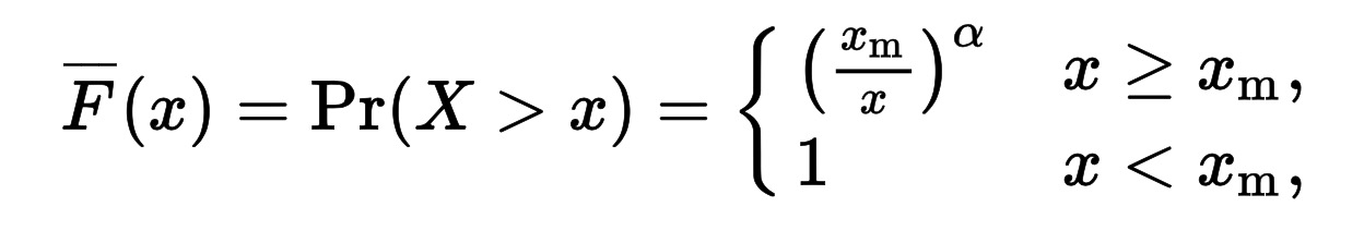
If X is a random variable with a Pareto distribution then the above formula gives probability that X will be greater than some number 

(source: wikipedia)
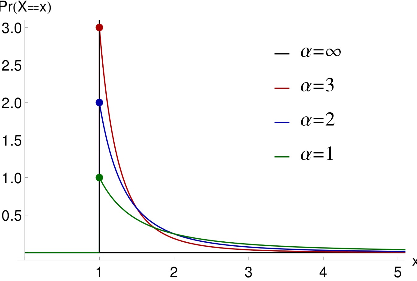
In the 80/20 rule, α is approximately 1.161.
Once again, the Pareto distribution tells us something about the relative distribution of large and small entities. Some of the many places it shows up, as listed in Wikipedia, include: the sizes of human settlements, file sizes, hard drive error rates, the values of oil reserves, sizes of sand particles, numbers of species per genus, and so on.
An alternative way of looking at the Pareto distribution is as follows:
The proportion of X with as least m digits (before the decimal point), where m is above the median number of digits, should obey an approximate exponential law, i.e., be approximately of the form c.10-m/α for some c, α > 0. In many cases, α is close to 1.
The adjacent possible and four examples
Now we can turn our attention back to the paper! The authors introduce a ‘mathematical model of the dynamics of novelties’ that is based on an idea called ‘the adjacent possible.’
Originally introduced in the framework of biology, the adjacent possible metaphor includes all those things, ideas, linguistic structures, concepts, molecules, genomes, technological artifacts, etc., that are one step away from what actually exists, and hence, can arise from incremental modifications and/or recombinations of existing material.
Here’s my intuition – imagine you’re wandering around the ‘land of the known.’ Most of the time you’re somewhere in the interior of the territory (and the larger the territory, the more likely it is that this will be so), but occasionally you find yourself at a border. There are no border signs, so you won’t necessarily know this is a border, but walking in a random direction from where you now are, you have a chance of venturing outside of the land of the known.
The model predicts the statistical laws for the rate at which novelties happen (Heaps’ law) and for the frequency distribution of the explored regions of the space (Zipf’s law), as well as the signatures of the correlation process by which one novelty sets the stage for another. The predictions of this model were tested on four data sets of human activity: the edit events of Wikipedia pages, the emergence of tags in social annotation systems, the sequence of words in texts, and listening to new songs in on-line music catalogs.
The model itself is based on ‘Polya’s Urns’…
Polya’s Urns
Consider an urn filled with 
These elements represent songs we have listened to, web pages we have visited, inventions, ideas, or any other human experiences or products of human creativity.
Let 
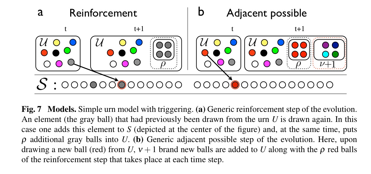
At each time step proceed as follows:
- Draw an ball
from the urn with uniform probability and add it to
- Put the ball
additional balls of the same colour. This part models the ‘rich get richer’ phenomenon making it more likely that we return to ball colours we have previously seen.
- If
new balls to the urn, each of a brand new colour. (Assume we have as many colours as we like, and can distinguish among them all!).
A variant of this process only adds the additional copies in step 2 if
The authors show that both variants of the urn model follow Heaps’ law for the number of distinct elements after t time steps, and a fat-tailed frequency rank distribution. It’s interesting because it shows how we can grow such a distribution step by step and thus potentially models how things grow in the real world. If you just wanted to generate a data set of a certain size (all at once) following the laws of real-world datasets I can think of easier ways.
By providing the first quantitative characterization of the dynamics of correlated novelties, these results provide a starting point for a deeper understanding of the adjacent possible and the different nature of triggering events (timeliness, spreading. individual vs. collective properties) that are likely to be important in the investigation of biological, linguistic, cultural, and technological evolution.
Social Physics
Alex Pentland runs a ‘Social Physics’ group at MIT, based at its core on a model of how ideas spread between people. Thus this model also offers some explanation for how a few things can become very popular, and others languish relatively unknown. Here’s the gist of the idea, taken from the 2014 Social Physics book.
Imagine a universe with 

}")
}")
The likelihood of a given observable action by person 
}|h_{t}^{(c)})")

}|h_{t-1}^{(1)},...,h_{t-1}^{(C)}) = \sum_{c=1}^{C} R^{c',c} \times P(h_{t}^{(c')}|h_{t-1}^{(c)})")


One of the most important consequences of this model is that it lets us take raw observations of behavior and gives us the social network parameters we need to get a numerical estimate of idea flow, which is the proportion of users who are likely to adopt a new idea introduced into the social network. (Social Physics, p83).